Import / export · raw data

Import a raw dataset

1. The Gallery screen shows the datasets with the thumbnails. The user can create a new folder and import images or import annotated data. The user can import data by clicking on the “Import Data” button.

   

2. Users can import data in two ways: by uploading images for model training or by generating synthetic (GenAI) defect data. Detailed information and import options for GenAI data are available on its dedicated page.

   

3. For Training, import data with the below options:

   • Import Images enables users to import files into a new imageset
   • Import Image Folders enables users to import folders with unannotated images
   • Import Annotated Dataset enables users to import annotated data in LabelMe, COCO, YOLO or Classification format
   • Import From ReliAudit imports audit images from ReliAudit
   • Create Empty Imageset enables users to import an empty imageset

4. When the user selects the “Import Images” option and clicks the “Import” button, the import process initiates.

   

5. The user should select images from the directory. Once images are selected, click on “Open”.

   

6. The imported data will be shown as a new dataset on the Gallery screen.

   

7. The user can check the images by double-clicking on the dataset folder. Users can:

   • Display images
   • Split datasets into training and test sets automatically with a random split or manually balance classes in train/test sets
   • Filter images to train/test/unassigned sets and statuses to annotated/not annotated
   • Select image for annotation

   

Import / export · annotated data

Import annotated data

1. The user can import data by clicking on the “Import Data” button.

2. Users can import data in two ways: by uploading images for model training or by generating synthetic (GenAI) defect data. Detailed information and import options for GenAI data are available on its dedicated page.

3. When the user selects the “Import Annotated Dataset” (1) option and clicks the “Import” (2) button, the import process initiates.

   

4. The user can select one of the following annotation formats:

   • LabelMe is the native format of Label Me
   • COCO is the common JSON format for machine learning
   • YOLO is the favored annotation format of the Darknet family of models
   • YOLOv3 is the third version of YOLO family formats
   • YOLOv4 is a format used with the PyTorch part of YOLOv4
   • YOLOv5 is a modified version of YOLO Darknet annotations
   • Classification imports image data organized in subfolders and automatically assigns each subfolder name as a label

5. Select any annotation format, then click on the “Import” button (e.g. Label Me).

   

6. The user should enter the folder directory. Once a file is selected, click on “Open”.

   

7. The imported data will be shown as a new imageset on the Gallery screen.

   

8. The user can check the annotated images by double-clicking on the imported folder. If any image is selected, the user can see the defined states and ROIs.

   

Import / export · export

Export data

1. Images and annotations can be exported from the dataset folder by using the “More” menu.

   

2. To export images, click the “Export Images” option, then simply select a folder to save images.

   

3. To export annotations, click the “Export Annotations” option, then select an annotation format (e.g. Label Me).

   

4. In the next step, select the desired annotation set(s) by clicking the check box (1). The “Export Images” radio button below gives users the choice to save annotations either with or without the corresponding images (2). Once selected, click on the “Export” button (3).

   

5. Select a folder from the directory to save annotations.

6. Annotations can also be exported from the image list page. To access this page, double-click on the dataset folder.

   

7. Click on the “Image Selection” check box to select images with the following options:

   • Select only this page
   • Select all images
   • Select ID range

   

8. Select any option from the list, then images will be selected. Right-click on the selected image(s) and select the “Export Annotations” option from the menu.

   

9. To export annotations, first select the annotation set(s). The user can select the “Export Images” option to export images and the “Add File Names” option to add file names to the exported data.

   

10. Then choose one of the formats below:

    • LabelMe
    • COCO
    • YoloDarknet
    • Yolov3
    • Yolov4
    • Yolov5

    

11. When the user selects any format and then clicks on “Export”, the export process initiates.

    

12. Choose a directory, then click on “Select Folder” to save the annotations.

    

13. The same process can be completed from the “Apply Operations” icon on the top-right.

    

14. Select “Export Annotations” options and complete the same steps.

    

15. Exported annotation files are shown in the designated directory.

    

Dataset operations

Extract ROIs

1. The Gallery screen shows the imagesets with the thumbnails. The user can extract ROIs of an image folder. Once extracted, the Gallery will display an image folder containing these ROIs. To export this folder, simply click on the “More” icon and select “Extract”.

   

2. Group names correspond to ROI groups within the imageset. By checking the checkbox “Group Name”, the user can export all ROI groups. The user can individually select ROI groups by clicking on the annotation set and then “Extract”.

   

3. Once extracted, the Gallery will display an image folder containing these ROIs.

   

4. The user can check the imageset by double-clicking on the imported folder. If any image is selected, the user can see the ROIs.

   

5. To export Regions of Interest as annotations, the user should click the “More” icon and select “Export Annotations”. Alternatively, ROIs can be exported as images by selecting the “Export Images” option. For more details, see Export data above.

   

Dataset operations

Merge and download datasets

In the Gallery screen, users are able to merge multiple datasets and/or download datasets from the server.

1. The user can merge imagesets by clicking on the “Merge” icon on the top-right.

   

2. Once clicked, select the desired image sets and specify the Merge output folder.

   

3. If the user clicks on the “Delete Input Imagesets” option, selected input imagesets will be deleted. Once all selections are done, click on the “Merge” button.

   

4. The merged imageset will be displayed in the gallery.

   

5. This page also allows users to download imagesets from the server by first entering the URL and choosing the desired data from the available choices.

   

   

   

6. Once selected, clicking “Next” will initiate the downloading process.

   

7. The new image set is added to the gallery. The user can check images by double-clicking on the image set folder.

   

Dataset operations

Process a dataset

1. Users can modify images by performing actions such as cropping, rotating and downsizing. Furthermore, images can be converted to grayscale and inverted using the “Process” feature. This feature is accessible by clicking on the “More” icon.

   

2. Enter the desired parameters or click the “Load Defaults” button to apply the default settings.

   

3. Once parameters are entered, click on the “Process” button.

   

4. The processed imageset can be reviewed in the Gallery.

   

Annotation

ROI annotation

The image annotation screen offers drawing and editing tools that enable users to manually annotate an image. These operations are carried out within the context of the currently displayed image. The user can:

• Navigate between images within an active image set
• Zoom and pan an image using CTRL + Mouse Wheel
• Generate regions of interest using basic shapes like rectangles and polygons
• Specify annotation sets and states for these regions of interest
• Choose distinct colors for each state by color picker
• Adjust existing regions of interest by modifying their properties (name, size, position, states), duplicating, or deleting them
• Create a parent-child hierarchy to semantically group regions of interest

1. In the Gallery, the user should select a dataset to initiate the annotation process.

   

2. The user can start the annotation by clicking any image from the image folder.

   

3. The right-side menu plays an essential role in the annotation screen, consisting of two primary sections: States and ROI List. The “States” section allows users to manage annotation sets; creating, editing or deleting them. Users can add states to any existing annotation set. To create a new annotation set, click “Add Annotation Set”.

   

4. To begin, define the annotation set (e.g. Scratch). Next, add the desired states (e.g. small, big) by clicking on “Add New Label” and then finalize the process by clicking “Create”.

   

5. Once an annotation set is created, the user can add a new state by clicking on the plus icon to include additional states.

   

6. A different color can be assigned to every component or state through the color picker.

   

   

7. The Annotation Toolbar is located horizontally at the top of the annotation screen. Each tool in the toolbar is represented by an icon. The user should select the “Draw” icon to create ROIs.

   

8. Based on the use case, the user can choose the appropriate annotation shape options below:

   • “Rectangle” is for area annotations
   • “Polygon” is for roughly or perfectly outlined annotations
   • “Whole Image” is for annotation without the region specification of the object
   • “Auto Polygon” is for automatically fitting the annotation to the defective area within a drawn rectangle

   

9. If the “Rectangle” option is selected, the user should define the ROI by drawing it.

   

10. If the “Polygon” option is selected, the user should define ROI by connecting straight lines.

    

11. Once an ROI is drawn, the user can select the appropriate state from the provided list.

    

12. Once all the ROIs in the current image are defined, the user can proceed to the next image by either clicking on the arrows at the top or by using the shortcut CTRL+D.

    

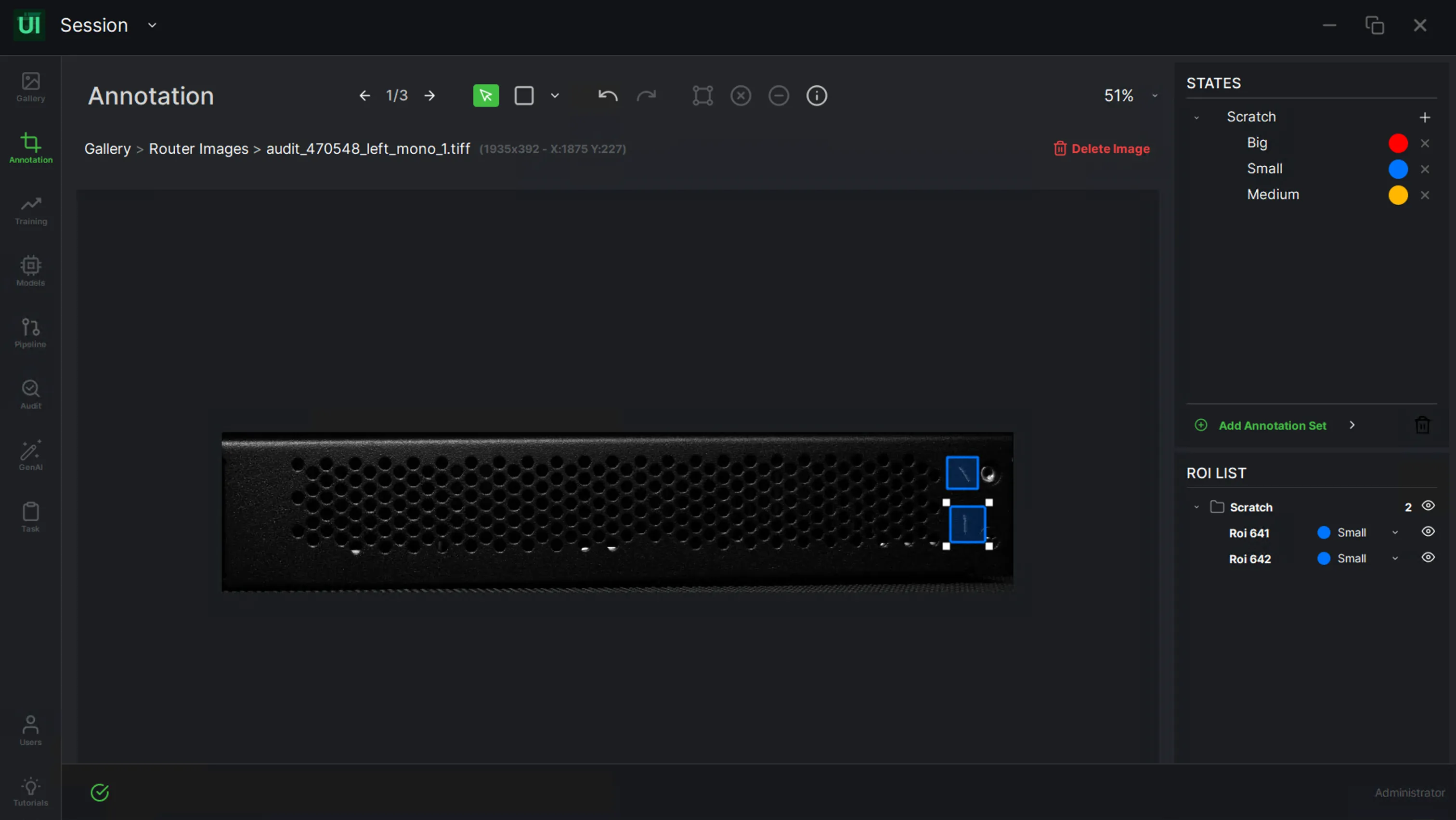
13. By clicking on any ROI, the user can modify its dimensions by adjusting its size as needed. Also, the user can delete an ROI by selecting and then pressing the “Delete” key on the keyboard.

    

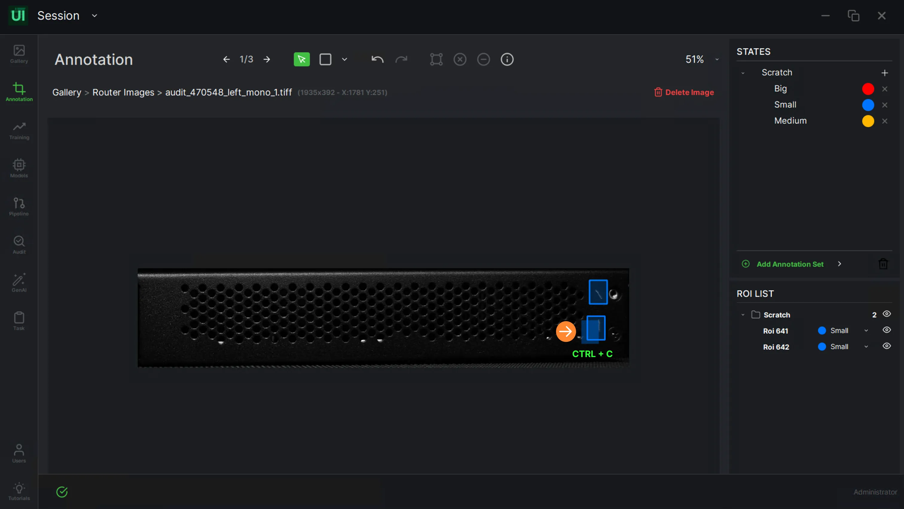
14. The user can copy and paste the same ROI by clicking on “CTRL+C”.

    

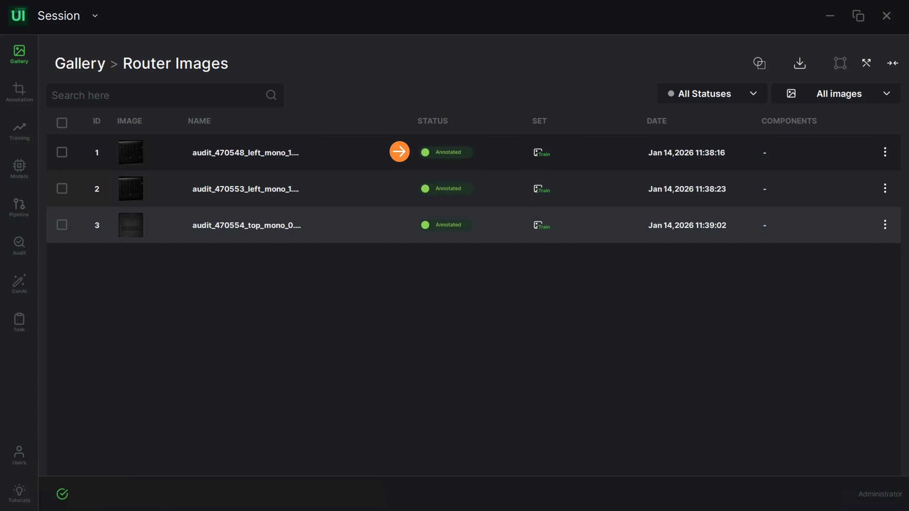
15. Once the annotation is completed, the image's status is automatically changed to “Annotated” in the status column.

    

Annotation

Whole image annotation

1. In the Gallery, the user should select a dataset to initiate the annotation process.

   

2. The user can start annotation by clicking any image from the image folder.

3. The user should select the “Whole Image” option to annotate the image without any region specification.

   

4. After choosing the “Whole Image” option from the annotation toolbar and then clicking on the image, a pop-up for states/components will appear. Simply click “Add Component” to continue with the annotation process.

   

5. First, the user should define the annotation set (e.g. Class) and add new states (e.g. Router), click on “Add New Label” and finally click on “Create”.

   

6. The user can change the color of the component through the color picker.

   

   

7. Once a “Whole Image” ROI is drawn, the user can select the appropriate defined state from the drawn box. Also, an ROI can be deleted by selecting and then clicking the minus icon in the top toolbar.

   

8. Once all the ROIs in the current image are defined, the user can proceed to the next image by either clicking on the arrows at the top or by using the shortcut CTRL+D.

   

9. Once the annotation is completed, the image's status is automatically changed to “Annotated”.

   

Annotation

Auto polygon

1. In the Gallery, the user should select a dataset to initiate the annotation process.

2. The user can start annotation by clicking any image from the image folder.

3. To create a new annotation set, click “Add Annotation Set”.

   

4. Enter an annotation set name (e.g. Scratch). Use the “Add New Label” button to include required states (e.g. small, big), then select “Create” to complete the setup.

5. For automated ROI generation, use the “Auto Polygon” tool. By drawing a rectangle around a defect, this tool automatically adjusts the annotation to fit the area's contours.

   

6. Once an ROI is drawn, the user can select the appropriate defined state from the provided list.

   

7. Once all the ROIs in the current image are defined, the user can proceed to the next image by either clicking on the arrows at the top or by using the shortcut CTRL+D.

   

8. Once the annotation is completed, the image's status is automatically changed to “Annotated”.

   

Annotation

Review and manage an annotated dataset

On the annotation page, users have the capability to manage, review and edit annotated images — loading new images, applying bulk operations, splitting and filtering for training, and editing ROI states.

Image management and display

1. To load new images locally, click on the “Load New Images” icon.

   

2. Select an image from the directory. Once an image is selected, click on “Open”.

   

3. The imported image will be shown in the image list.

   

4. “Apply Operations” allows the user to perform multiple operations. To enable this function, the user should choose “Only this page” or the “Select all images” option to select images.

   

   

5. Similarly, if the user clicks on the “More” icon on the right, a dialog box will be displayed containing functions similar to “Apply Operations”.

   

6. Once the “Apply Operations” dialog box is displayed, the user can:

   • Duplicate or Delete images
   • Export Annotations
   • Assign images to train and test sets
   • Move images to another dataset by selecting Move to Another Imageset

   

Prepare for training and filter images

1. “Split Images” allows the user to split images before the training as Train/Test Sets with three options.

   

2. As the dataset is split, the image status will change from “Unassigned” to “Train/Test Sets”.

   

3. “Clear Sets” allows the user to clear all the current statuses. The new statuses of the images will change to Unassigned Set.

   

   

4. The “All Statuses” option enables the user to filter images based on “Annotated” or “Not Annotated” statuses. Upon selecting either of these options, the list view will be automatically updated to reflect the chosen filter.

   

5. “All Images” allows the user to filter the images by selecting Train/Test/Unassigned statuses. Upon selecting either of these options, the list view will be automatically updated to reflect the chosen filter.

   

Annotation operations

1. To annotate an image, either double-click on it or right-click and select “Annotate”.

   

2. Export annotations either by right-clicking on the image or by selecting the option from the Apply Operations menu. For more details, see Export data above.

   

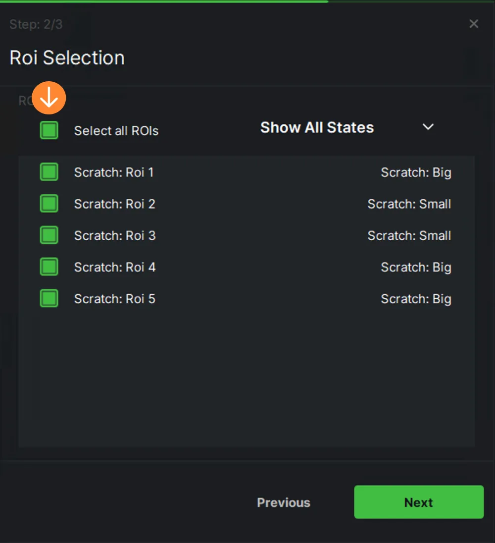
3. In the image list, “Edit ROIs States” allows the user to change the state of ROIs. From the available “ROI Groups”, the user can make the selections; when the annotation set is chosen (e.g. Scratch), click “Next” to proceed. When the “Select all ROIs” checkbox is marked, it allows the user to choose all ROIs collectively — alternatively, specific ROIs can be individually selected or deselected from the list. Then select a defined state from the list to designate it as the new ROI for your dataset and select “Copy” to apply the assignment.

   

   

   

   

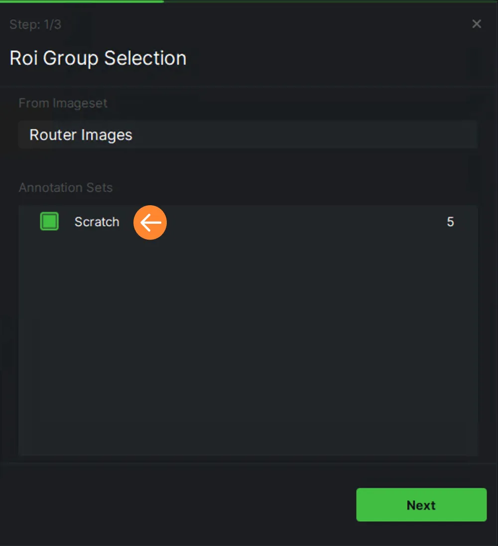
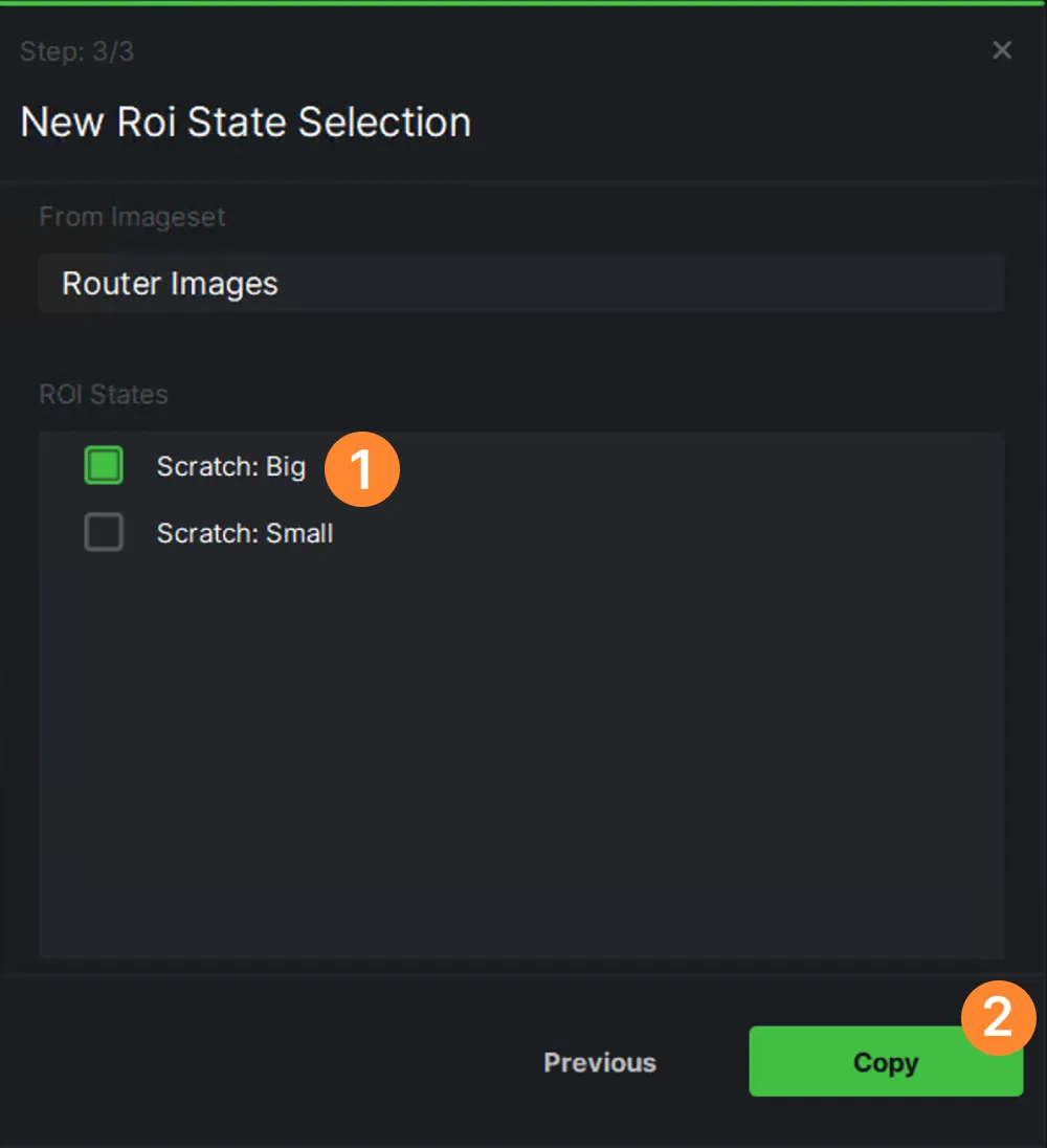
4. Following this update, the dataset will reflect the new state or states, which you can then verify within the ROI list.

   

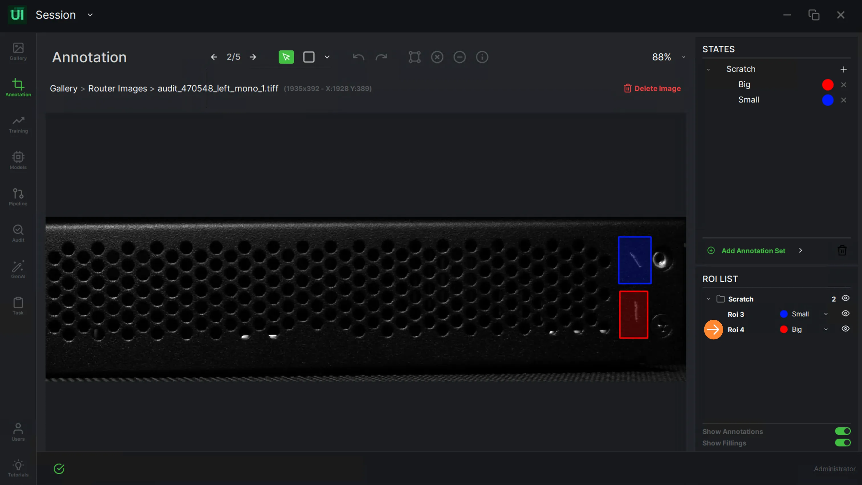
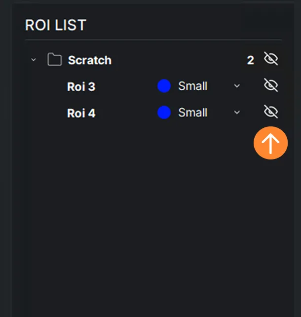
5. The user can change the ROI states by selecting options from the dropdown menu.

   

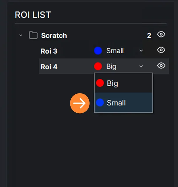
6. Switch the visibility of these ROIs by clicking on the “View” icon.

   

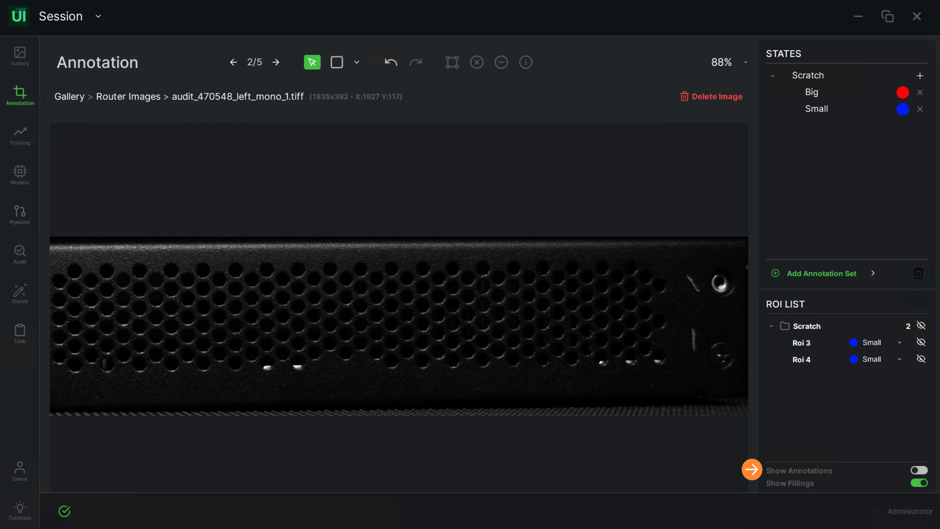
7. The “Show Annotations” switch button allows the user to show or hide annotations.

   

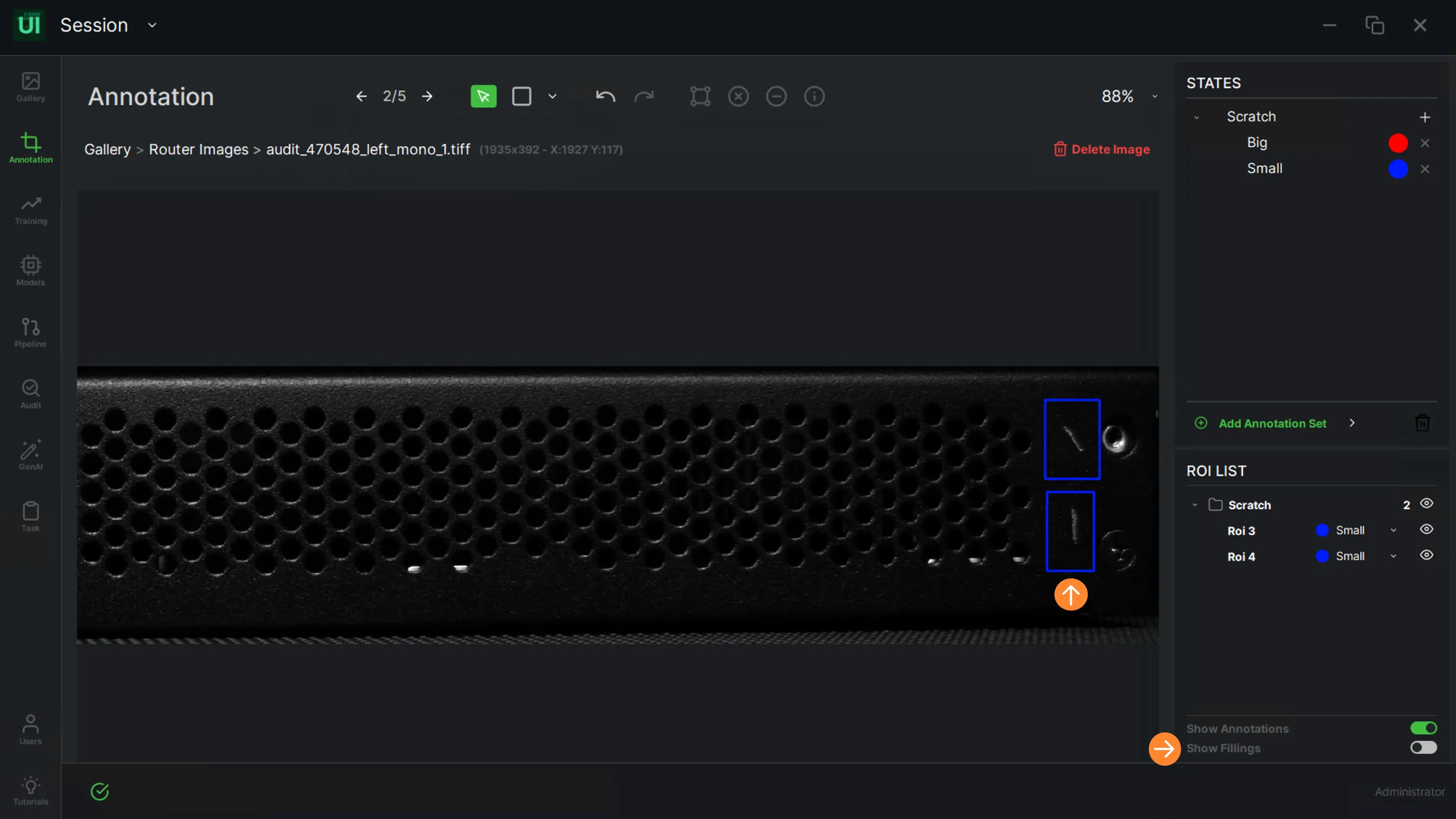
8. The “Show Filling” switch button allows the user to show or hide ROI fillings. If the fillings are hidden, only the edges will be displayed.

   

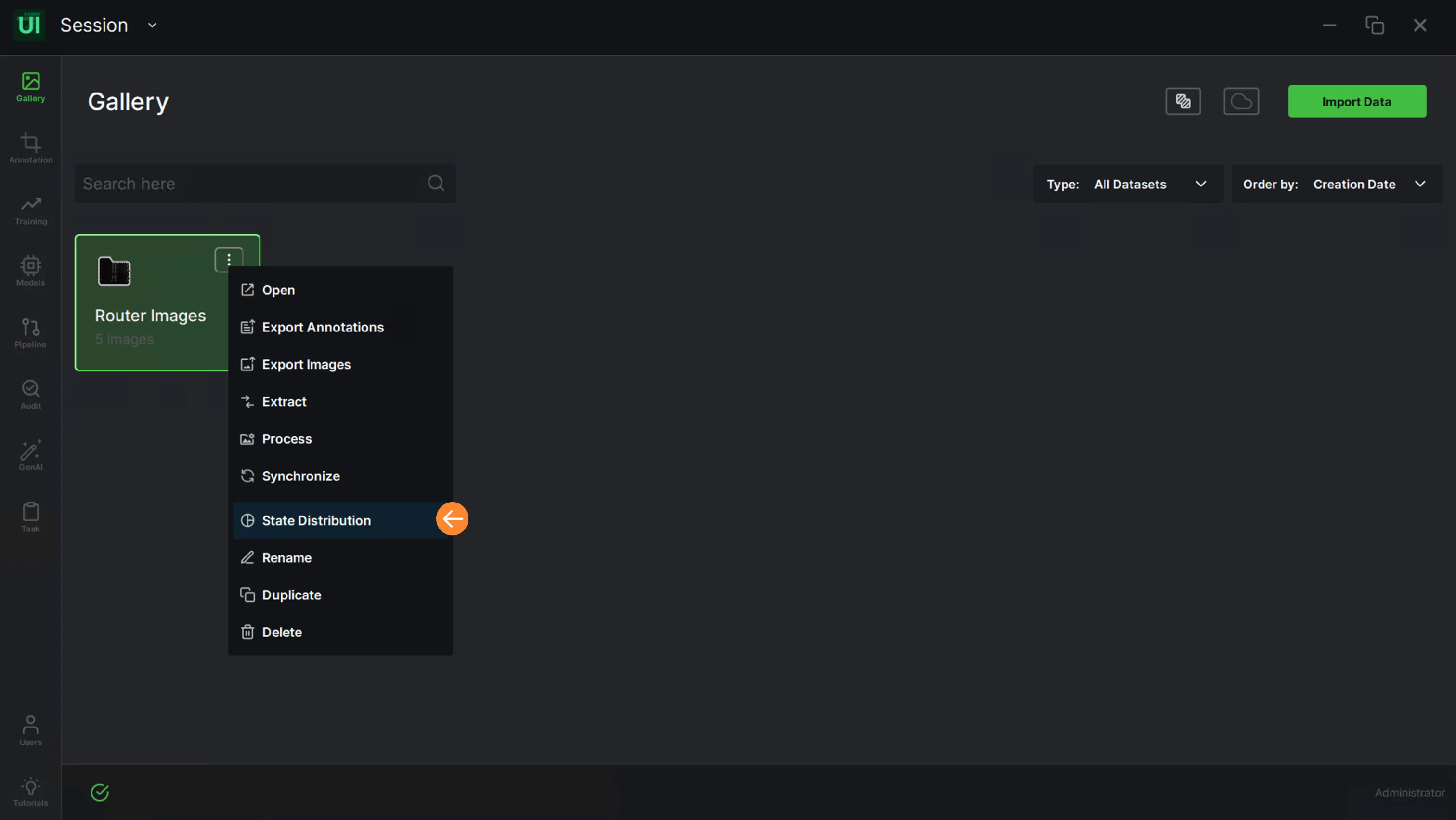
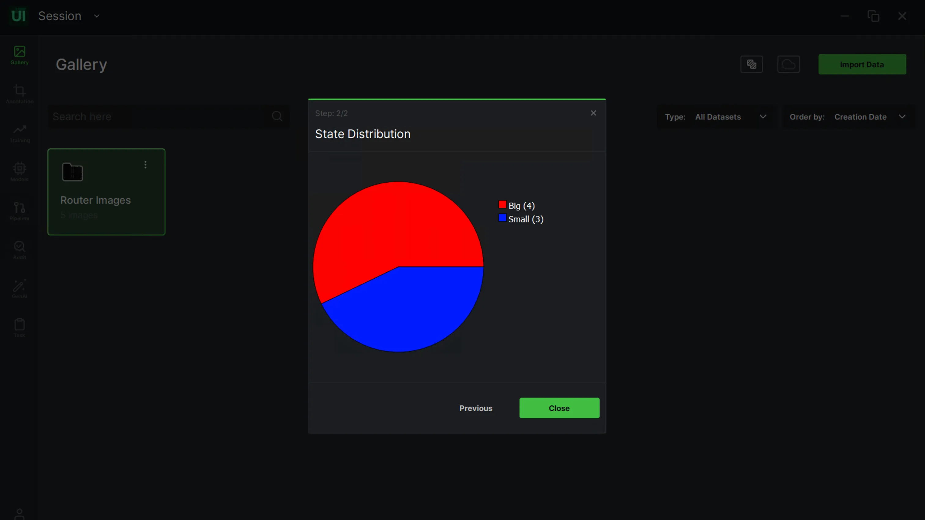
9. Finally, use the “More” icon of an annotated dataset to examine the distribution of states.

   

   

GenAI

Defect library

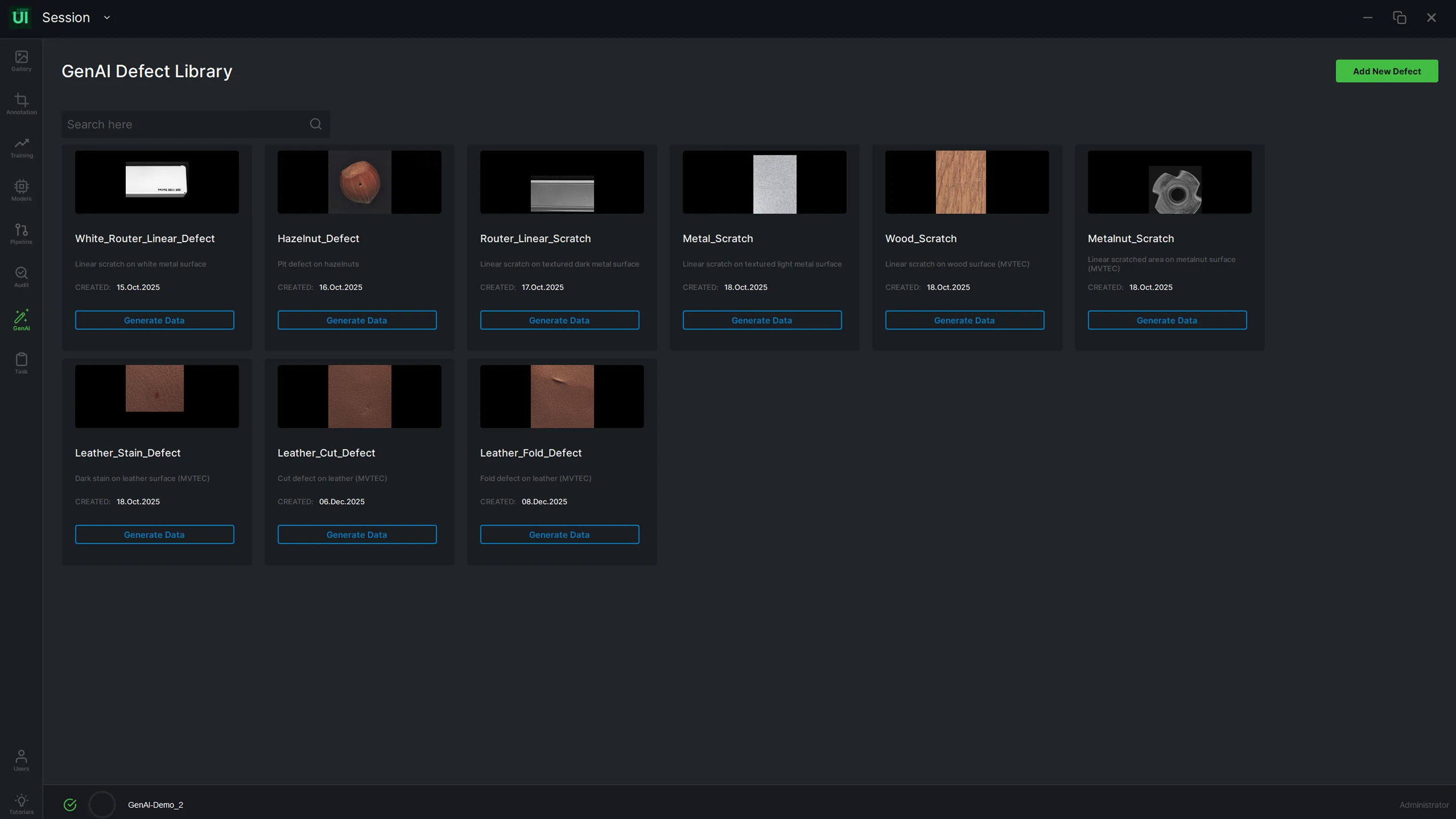
1. ReliVision provides a continuously evolving defect library, allowing users to add their own defects and generate additional data.

   

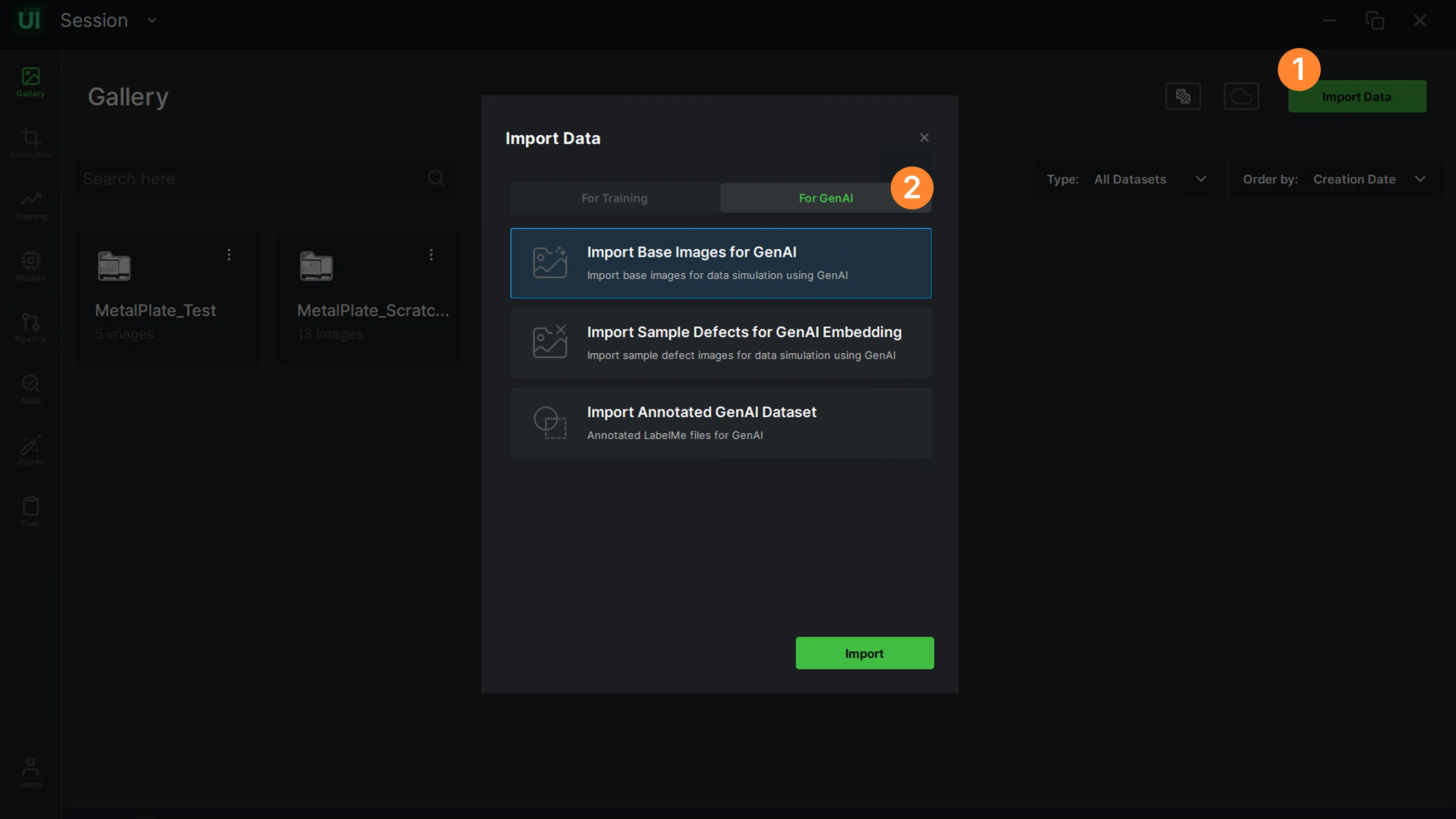
2. To create a new defect, the user can start with importing defect images from the Gallery. Click on the “Import Data” button (1), then select the “GenAI” tab (2).

   

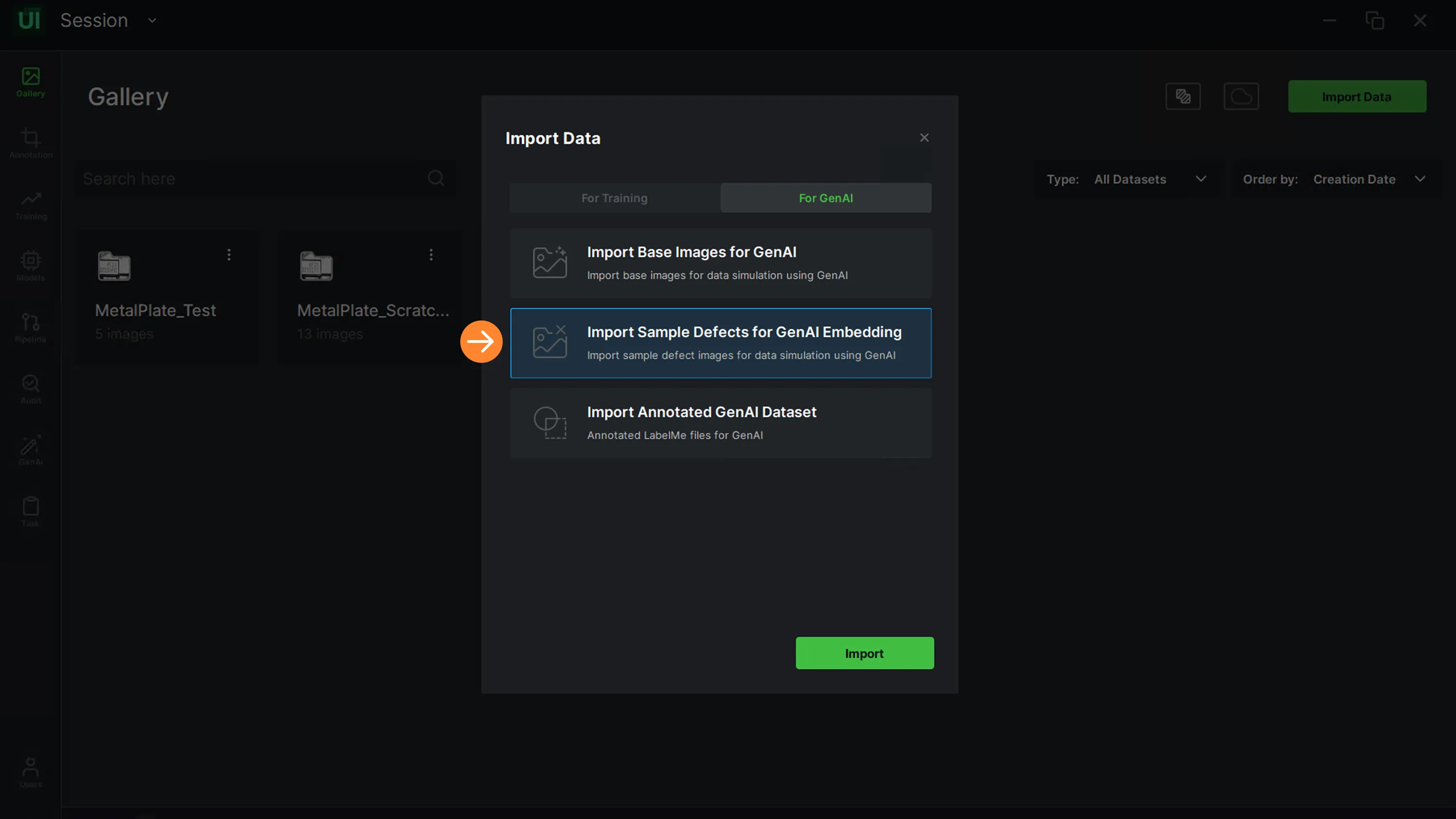
3. In the GenAI tab, the user can:

   • Import Base Images for GenAI
   • Import Sample Defects for GenAI Embedding
   • Import Annotated GenAI Dataset

4. Select the “Import Sample Defects for GenAI Embedding” option.

   

5. Select defect images from the directory, then click on “Open”.

   

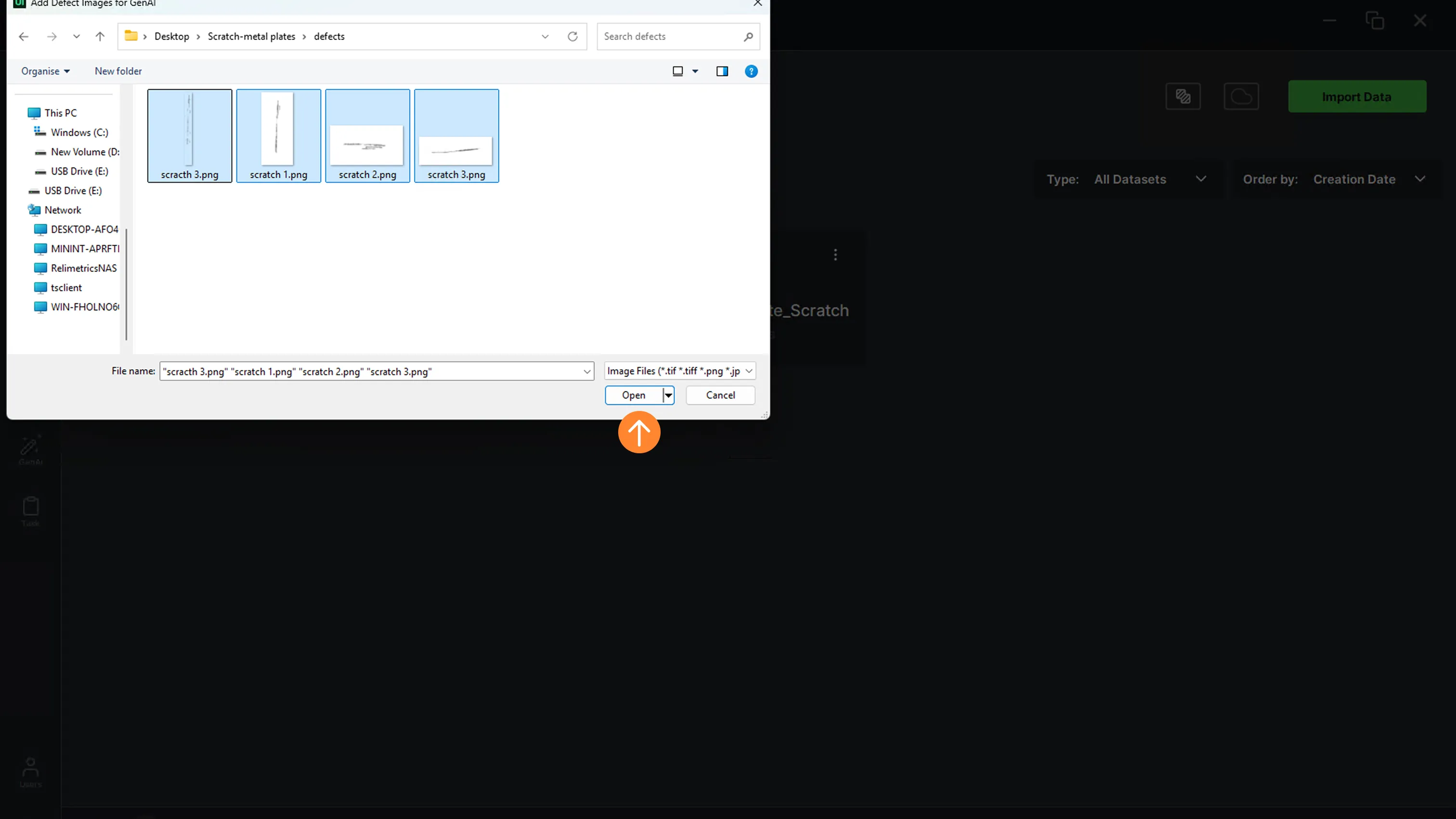
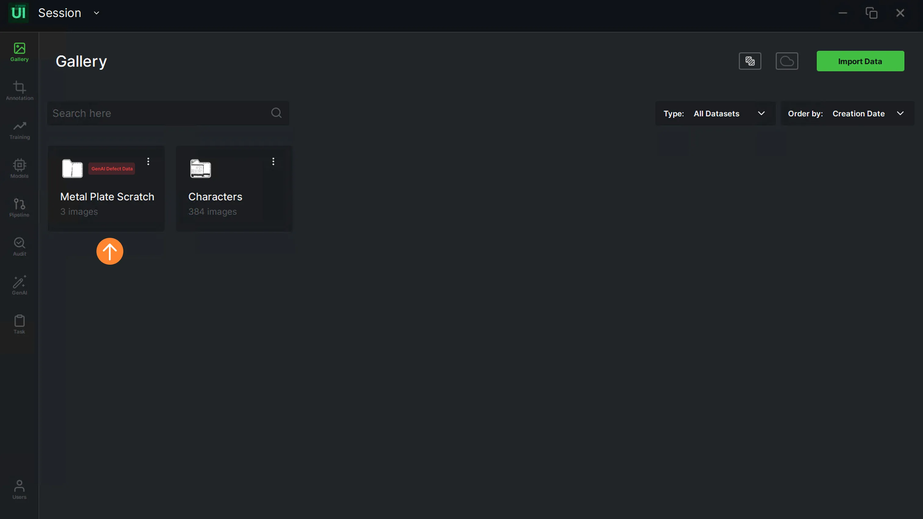
6. Once the images are imported, open them in the Gallery.

   

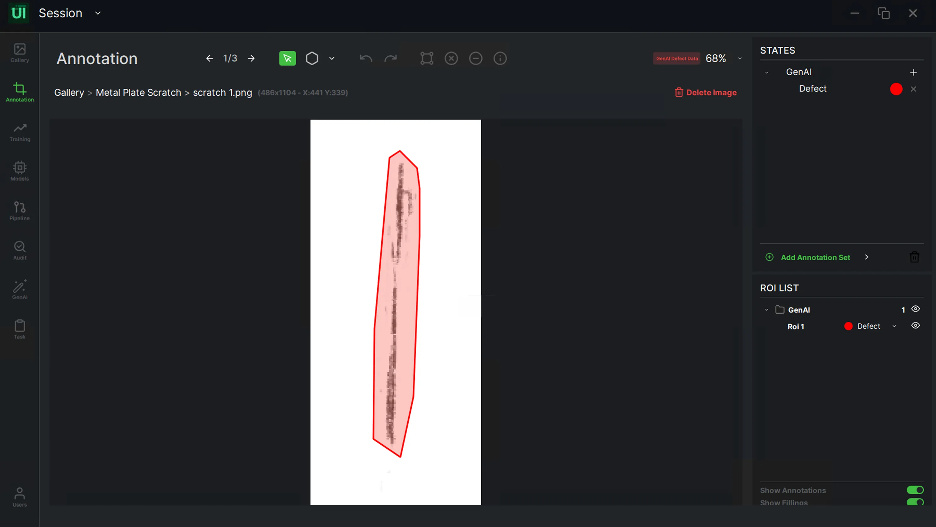
7. Annotate the defected area. For more details about annotation, see ROI annotation above.

   

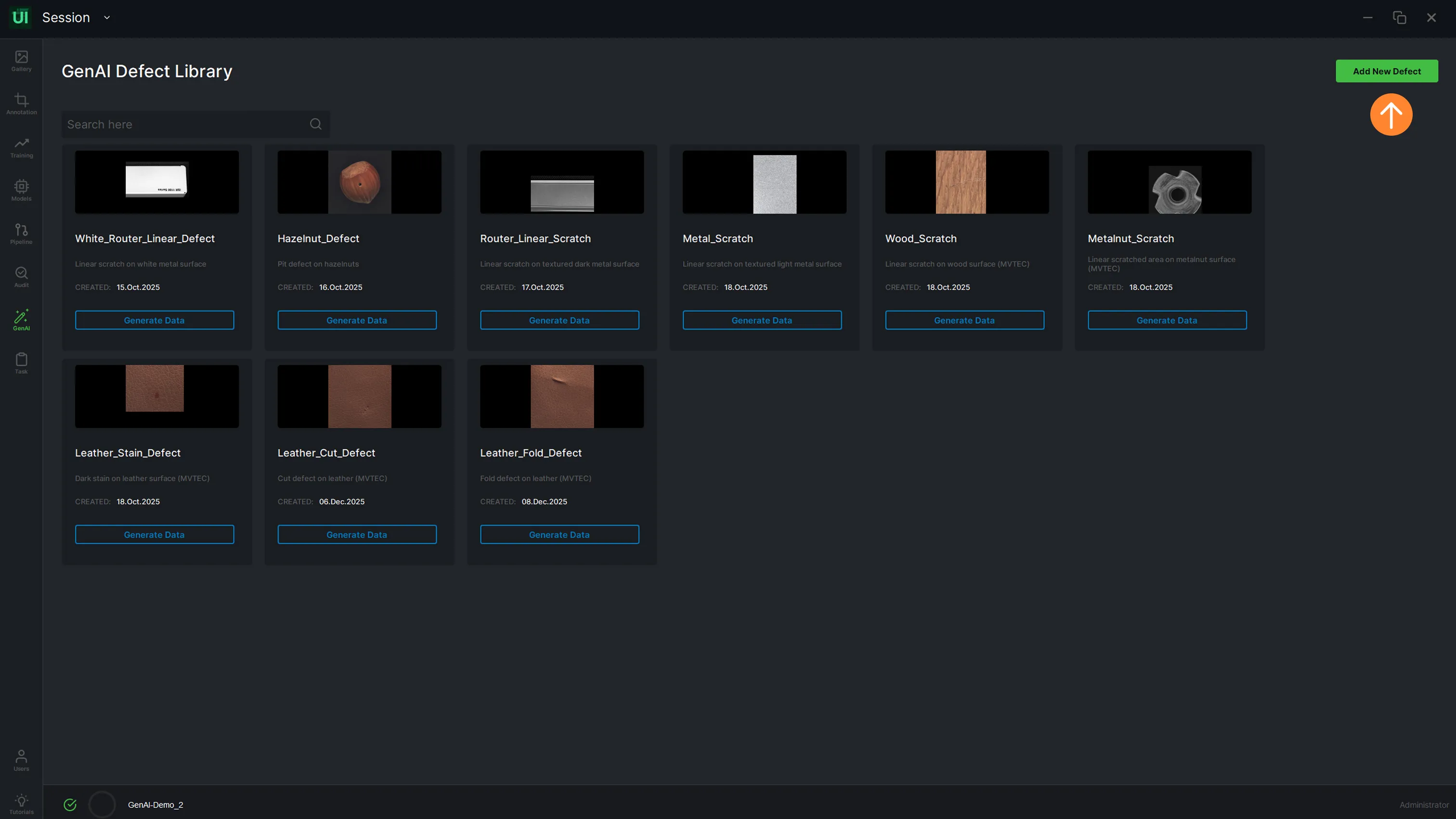
8. Once all defects have been annotated, the user can go to the GenAI page and click on the “Add New Defect” button.

   

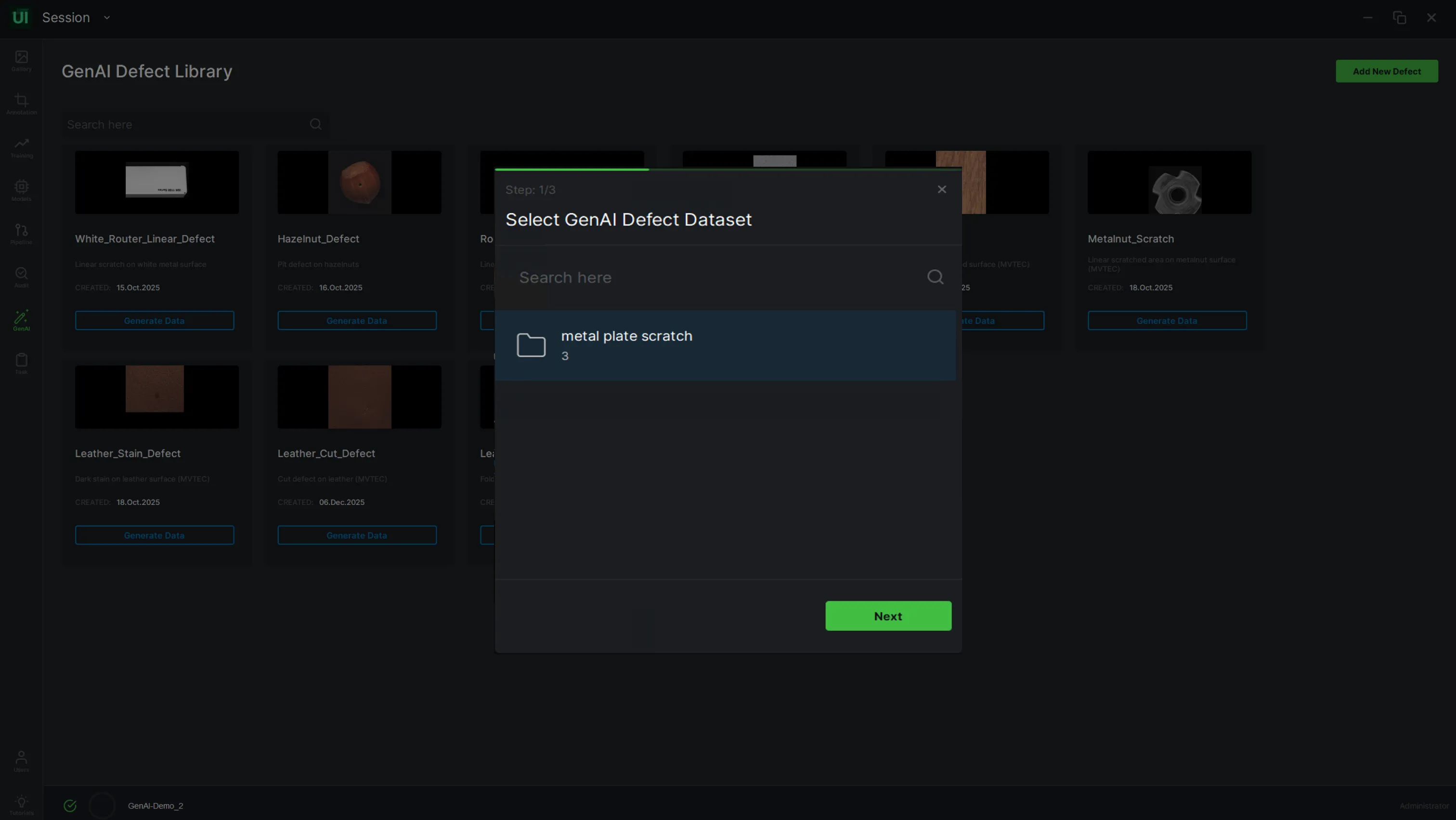
9. Select the GenAI defect dataset (e.g. metal plate scratch), then click “Next”.

   

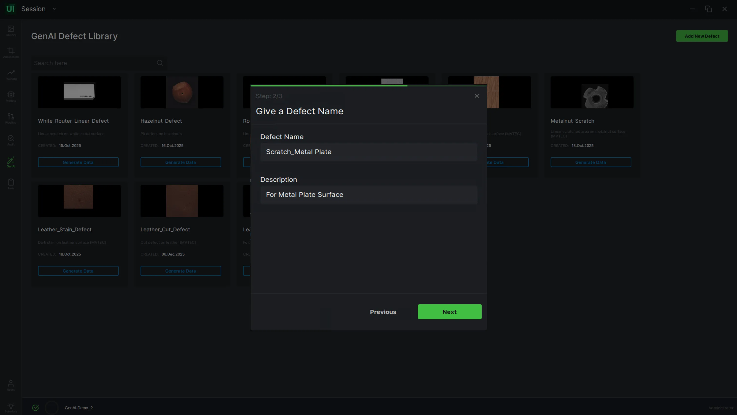
10. Give a defect name (e.g. Scratch_Metal Plate), add a description (optional), then synchronize the data.

    

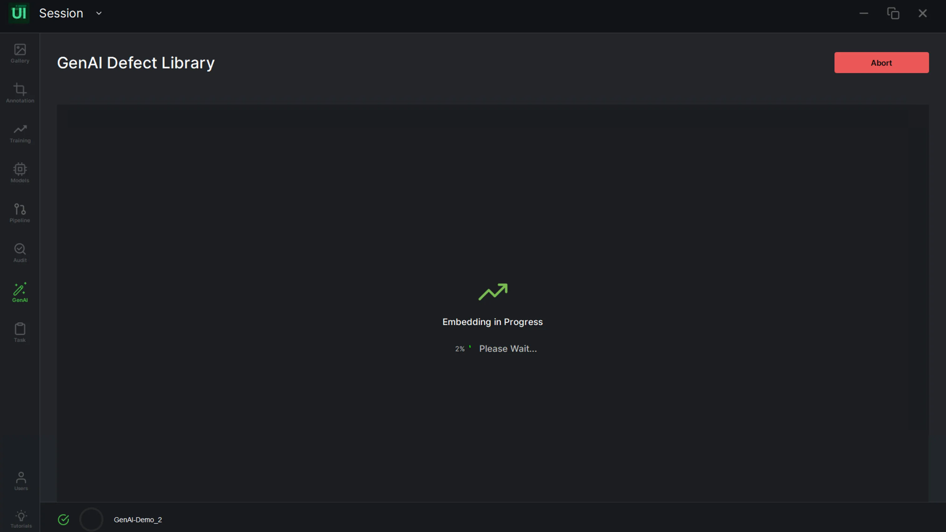
11. Please note that defect embedding may take hours.

    

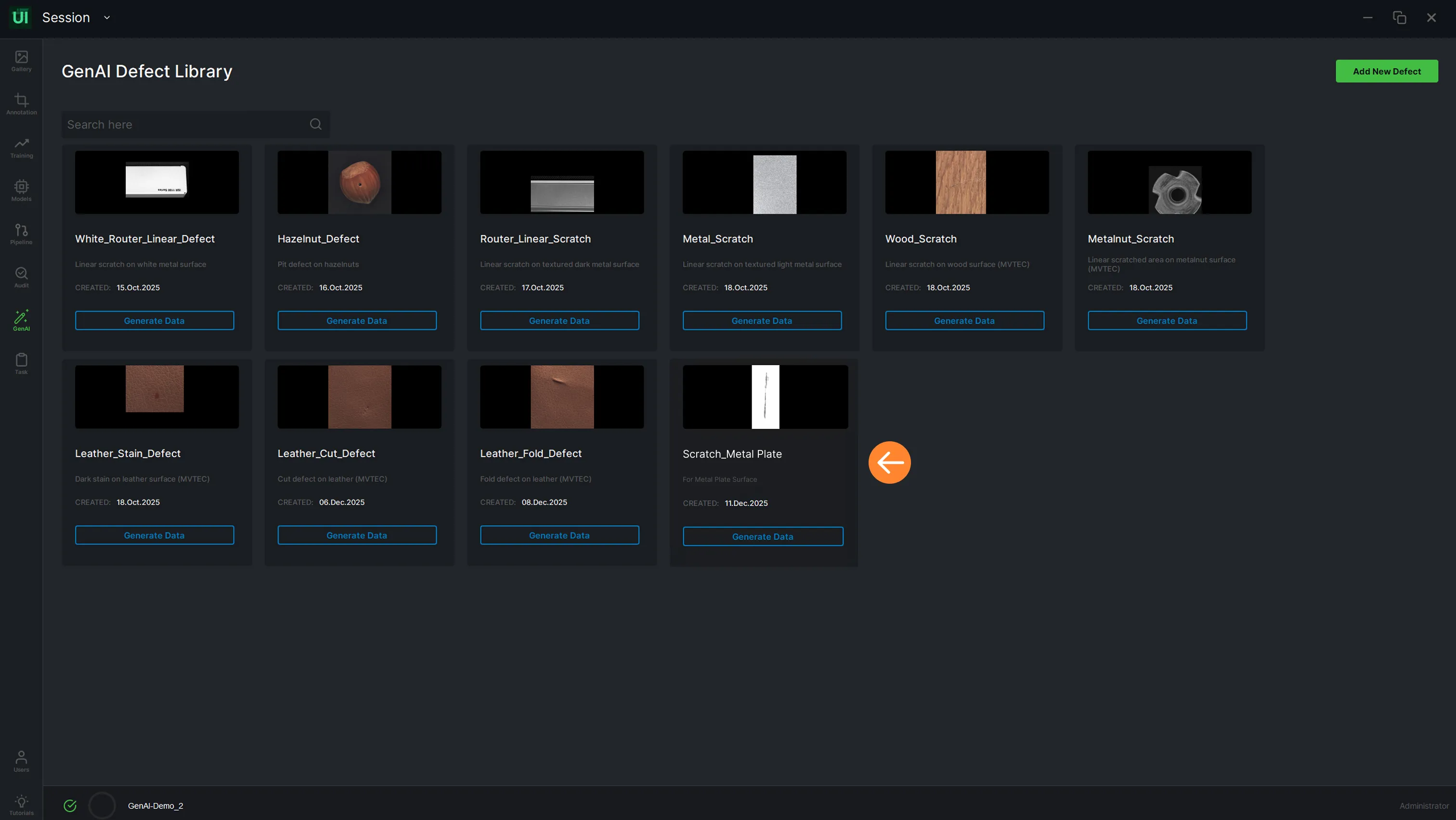
12. Once it is finished, the new defect type can be reviewed in the Defect Library.

    

GenAI

Synthetic data generation

1. For synthetic data generation, the user can start with importing base (OK) images from the Gallery. Click on the “Import Data” button (1), then select the “GenAI” tab (2).

   

2. Select the “Import Base Images for GenAI” option.

   

3. The imported dataset can be checked in the Gallery.

   

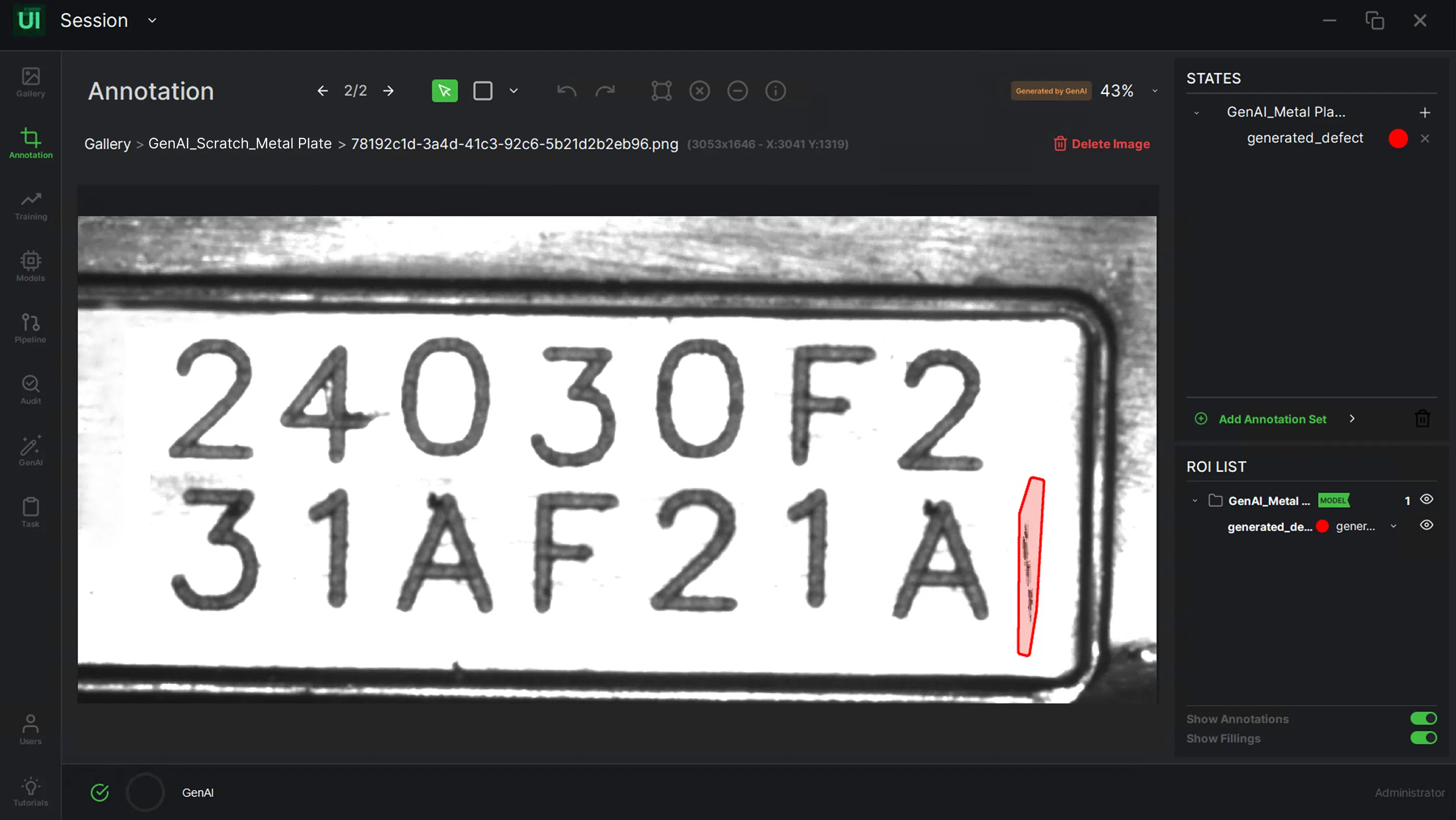
4. The user should use the annotation tool to mark the areas where they want to add defects. Also non-defective areas can be annotated if needed. For more details about annotation, see ROI annotation above.

   

5. Once annotation is complete, navigate to the GenAI page. Click on the “Generate Data” button on the selected defect.

   

6. Choose a GenAI base (OK) dataset (e.g. metal plate ok images).

   

7. Enter a name for the new dataset (e.g. GenAI_Scratch_Metal Plate).

   

8. The user can specify the number of defective images for data generation.

   

9. Within the “Advanced Options” menu, the “Preserve Color” (1) check box enables the application of the defect’s native coloration to the surface area. The “Blending Strength” (2) setting facilitates a more natural alignment between the defect and background lighting; note that higher values can result in a more translucent defect appearance.

   

10. The user can automatically set defect dimensions by selecting the “Load Defaults” option, or choose to refine these size parameters manually. To ensure accuracy, the preview tool enables users to visualize the precise area designated for the defect on the image.

    

11. After synchronizing the dataset, click on the “Generate” button.

    

12. Go to the “Gallery” page to review newly generated images. These synthetic images can be used for training.

    

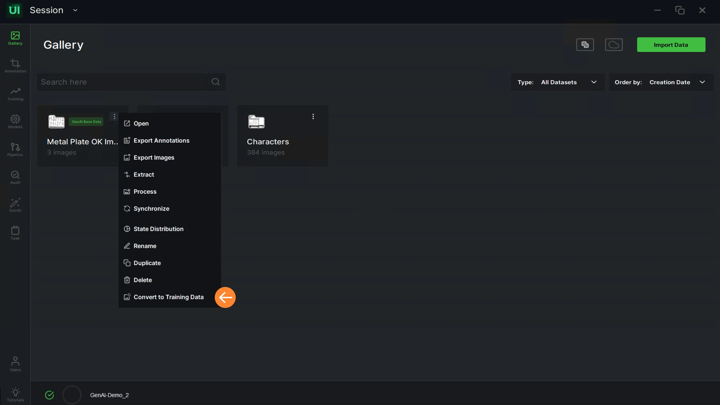
13. Additionally, base defected or OK datasets for GenAI can be used for training. Click on the “More” icon and select the “Convert to Training Data” option.

    

Training · from scratch

Training an AI block

1. In the Gallery screen, the user can check the images and the annotations before starting the training.

   

2. In the left menu, go to “Training” and click on “Start New Training” to train the model from scratch.

   

3. The user has two options as a roadmap:

   • “First Training” enables users to develop a new model from the beginning.
   • “Fine-Tuning of an Existing Model” is utilized for optimizing and retraining models to enhance precision.

   

4. A Training Type should be selected from the options below:

   • “Detection” is utilized in the process of identifying and categorizing object regions
   • “Classification” is utilized for classifying regions of interest (ROIs)
   • “Semantic Segmentation” is utilized to precisely detect object shapes
   • “Anomaly Detection” is utilized to identify irregularities in the input images

5. If an object detection model will be trained, the user should choose “Detection”. After selecting it, click on “Next” to proceed.

   

6. If the imageset hasn't been split previously, it should be divided into a Train Set and a Test Set at this stage. Once the split is completed, the user can proceed by clicking the “Next” button.

   

7. The user must ensure that data annotation is completed before beginning the training process, as unannotated datasets will prevent the finalization of the model.

   

8. After selecting the annotation set, click on “Next”.

   

9. Verify that the state distribution aligns with defined annotations, then proceed by clicking “Next”.

   

10. Detecting the optimal architecture for the training is done automatically. Settings can be reconfigured from “Advanced Options” if needed.

    

11. Within the “Advanced Options”, users have the following selections available:

    • “ReliNetDet-Max”: provides a faster network configuration.
    • “ReliNetDet-Medium”: optimized for standard, normal-sized networks.

    After making your choice, click the “Next” button to proceed.

    

12. The user should define a model name (e.g. Scratch_Detector) according to the use case, then click on “Next”.

    

13. The “Load Defaults” button allows the user to set the training parameters automatically. Additionally, the user has the option to input custom parameters manually.

    

14. The user can select the “Tiling” option to divide an image into smaller sections or tiles. This is useful for handling large images and improving data processing performance. The “Stratified Tiling” option temporarily uses class-balanced train/test splitting instead of random splitting.

    

15. The “Advanced Options” menu allows for the modification of training parameters, including resolution, initial learning rate, momentum and weight decay.

    

16. The user should synchronize the data before training by clicking the “Synchronize” button. After the synchronization process finishes, click the “Start Training” button.

    

17. In the Status tab, Model Loss and Mean Average Precision plots can be checked in real time.

    

    • Model Loss Curve: a graphical representation that illustrates how the loss of the model changes over epochs during both the training and validation phases. The loss curve provides valuable insights into the model's performance and convergence throughout the training process
    • Training Loss Curve: shows how the loss decreases during the training phase. It provides information on how well the model is fitting the training data (blue curve)
    • Validation Loss Curve: shows how the loss changes during the validation phase, using data that the model hasn't seen during training. It helps assess the model's generalization ability (green curve)
    • mAP: the mean or average of the AP values calculated for each object class. It provides a single measure of the model's performance across all object classes. Higher mAP values indicate better overall performance
    • Accuracy: measures how often the model correctly identifies objects (both true positives and true negatives) out of all objects present in the image. It is the ratio of correct predictions to the total number of predictions

18. The user can monitor the progress of the training by checking the Status bar.

    

19. Once the training has finished, click on the “Evaluation” tab to see the training statistics: total number of images, accuracy and mean IoU.

    

20. Mean IoU can be changed by moving the slider.

    • “Mean IoU” is the average of IoUs
    • “IoU” measures the overlap between the predicted bounding boxes and the ground truth bounding boxes
    • The mispredicted images and their corresponding Mean IoU scores are displayed in the table view

    

Training · retraining

Fine-tuning (retraining)

Retraining within the ReliVision platform enables QA teams to quickly adapt models to new defects, changing conditions and evolving production needs without external dependency. This ensures continuous accuracy and performance while significantly reducing downtime and iteration cycles.

1. Before starting, ensure you are using an up-to-date model — models trained with version 4.0.0 are not supported for fine-tuning. Then click the “Train New Model” button in the top right.

   

2. As a roadmap, select “Fine-Tuning” and click “Next”.

   

3. Fine-tuning scenarios include the options below:

   • “Continue Training Beyond Initial Epochs” is used to improve a model using the same dataset. It is ideal when the model performs well but can still benefit from incremental optimization.
   • “Add New Data to an Existing Model” is used to enhance a model with additional labeled data. It is useful when new defect types appear or when edge cases need better representation.
   • “Adapt a Trained Model to a New Dataset” is used to apply an existing model to a different but related dataset. It is ideal for scaling efficiently across similar use cases or production lines.

   Select any of them, then click on “Next”.

   

4. Select the Training Type (e.g. Detection) and click on “Next”.

   

5. Select the existing model (e.g. scratch detector) and click on “Next”.

   

6. Select the imageset. If the imageset hasn't been split previously, it should be divided into a Train Set and a Test Set at this stage. Once the split is completed, proceed by clicking the “Next” button.

   

7. Select the annotation set and verify the state distribution.

   

8. Detecting the optimal architecture for the training is done automatically. Settings can be reconfigured from “Advanced Options” if needed.

   

9. The user can select between the “Advanced Options” options:

   • “ReliNetDet-Max” can be chosen for the fastest and best performing configuration.
   • “ReliNetDet-Medium” can be chosen for a normal-size network.

   Once it is selected, click on “Next”.

   

10. The user should define a model name (e.g. Scratch_Detector 2), then click on “Next”.

    

11. The “Load Defaults” button allows the user to set the training parameters automatically.

    

12. Additionally, the user has the option to input custom parameters manually in Advanced Options.

    

13. Data should be synchronized before retraining by clicking on the “Synchronize” button. When the data synchronization is done, click on the “Start Training” button.

    

14. In the Status tab, Model Loss and Mean Average Precision plots can be checked in real time.

    

15. Once the training has finished, click on the “Evaluation” tab to see the training statistics: total number of images, accuracy and mean IoU.

    

Training · prediction

Running an AI block

The user has the capability to execute any trained AI model on available datasets within the Gallery. Prediction outcomes are immediately accessible for evaluation and are automatically saved to the imageset under the corresponding model's name for subsequent review and reference. This functionality is available through ReliUI's prediction screen.

1. In the training screen, the “PREDICTION” tab enables the user to start a testing process on a model by simply clicking on the “Start” button.

   

2. The user should select a model for prediction and click on “Next”.

   

3. The user should select the imageset that will be used for prediction and then click on “Next”.

   

4. Before initiating a prediction, ensure the data is updated by clicking the “Synchronize” button. Once the synchronization process is complete, select “Start Prediction” to begin.

   

5. The user can review the model's prediction results by checking the list of images on the left side along with the corresponding region predictions and their respective precision values on the right side.

   

6. The “Show ROIs” switch button on the bottom allows the user to show or hide annotations.

   

7. By clicking the “Save” icon located at the top, prediction results can be stored directly within the dataset chosen for testing.

   

8. Prediction results alongside the annotations can be reviewed from the Gallery, by clicking on the dataset. The image displays both the predictions and the annotations, which are clearly marked.

   

9. In the “STATES” column, the user can check the defined classes alongside the prediction results generated by the trained model (e.g. scratch_detection).

   

10. To examine detailed performance metrics, users can select the “Statistics” icon at the top of the screen. This feature provides a comprehensive overview of the confidence distribution in the total image count.

    

Training · comparison

Review models

On the “Review Models” page, trained models and their performances can be compared. Models can be filtered by type, creation date or name. Key metrics such as validation accuracy, validation loss and resolution can be reviewed, while the Model Loss and IoU graphs can also be saved as images.

1. The Models page provides an organized overview of trained models, including their types, source datasets, number of classes and architectures, ensuring ease of use for the user.

   

2. Models can be filtered by their type simply by clicking on the “All Types” dropdown menu. Once it is selected (e.g. detection), the list will be updated.

   

3. Models can be sorted by their creation date or name.

   

4. The “More” menu allows users to:

   • Export Model
   • View Source Data
   • Delete Model

   

5. The user can review more details about the model by clicking on the “Details” button.

   

6. The details page provides an overview of the model's key validation results and configurations. Users can review the resolution value, tiling option (whether it's on or off) and the total number of classes. Additionally, the page features graphical representations of the model's performance, including “Model Loss” and “Intersection Over Union (IoU)” graphs.

   

7. To save a graph view as an image, click the “Save” icon (1) and select the desired directory (2).

   

Pipeline editor

Create and edit a pipeline

1. In the main screen of the Pipeline Editor, the user can create new pipelines. Simply click on “Create New Pipeline”.

   

2. Enter a Pipeline Name (e.g. Character Detection) and specify the Purpose/Task (optional).

3. The generated pipeline will be presented as a folder. To access the pipeline editor screen, simply double-click on the folder.

   

4. The Pipeline Editor page is composed of three main sections:

   • Left menu (1)
   • Main action area: “Run Pipeline”, “Move to ReliAudit” and “Take Screenshot” buttons (2)
   • Workflow area (3)

   

5. The pipeline's left menu covers the following functions:

   • Source imageset / Output imageset
   • AI Models
   • Branching
   • Predictions
   • OCR
   • Image Processing

   

6. To return to the list of pipelines, the user can simply click on the “Pipeline Editor” title in the navigation menu.

   

7. The user can drag and drop any node from the left menu and compose any pipeline by connecting these blocks with the output nodes.

   

8. The “Source Imageset” node requires synchronization before using its data in the Pipeline Editor. Go to the Gallery and click “Synchronize” from the “More” menu to send the image set to the server.

   

9. Go back to the Pipeline Editor to continue. The user has the flexibility to select either a single model or a combination of models tailored to their specific use case. The menu displays four model categories for each task, namely:

   • Detection
   • Classification
   • Semseg (Semantic Segmentation)
   • Anomaly Detection

   

10. For most AI models (excluding Classification), users can fine-tune performance by adjusting the “Recall” and “Precision” settings.

    • Increasing Recall reduces the miss rate (fewer true positives are missed) but may lead to more false detections.
    • Increasing Precision decreases the number of false detections, but this can result in an increase in the miss rate (more true positives are missed).

    

11. For a single model scenario, drag and drop “Source Imageset” along with either the “Detection Model”, “Classification Model”, “Semantic Segmentation” or “Anomaly Detection” nodes depending on the defined task.

    

12. The user must select the appropriate model from the available options under the “Select Model” dropdown along with the source imageset.

    

13. To create a combined pipeline, such as one featuring both a detector and a classifier, the user must connect three specific individual nodes: “Source Imageset”, “Detection” and “Classification”. To connect different types of models, the “Generate Output” option must also be enabled (e.g. on the Detection model).

    

14. Click on the “Run Pipeline” button to execute the pipeline.

    

15. The prediction outcomes are visible in the training section, specifically under the “Prediction” tab, enabling users to evaluate the pipeline's performance. To store the pipeline results as ROIs on the dataset, select the “Save” icon.

    

16. Go to the Gallery and access the dataset associated with the specified pipeline to review and compare performance results.

    

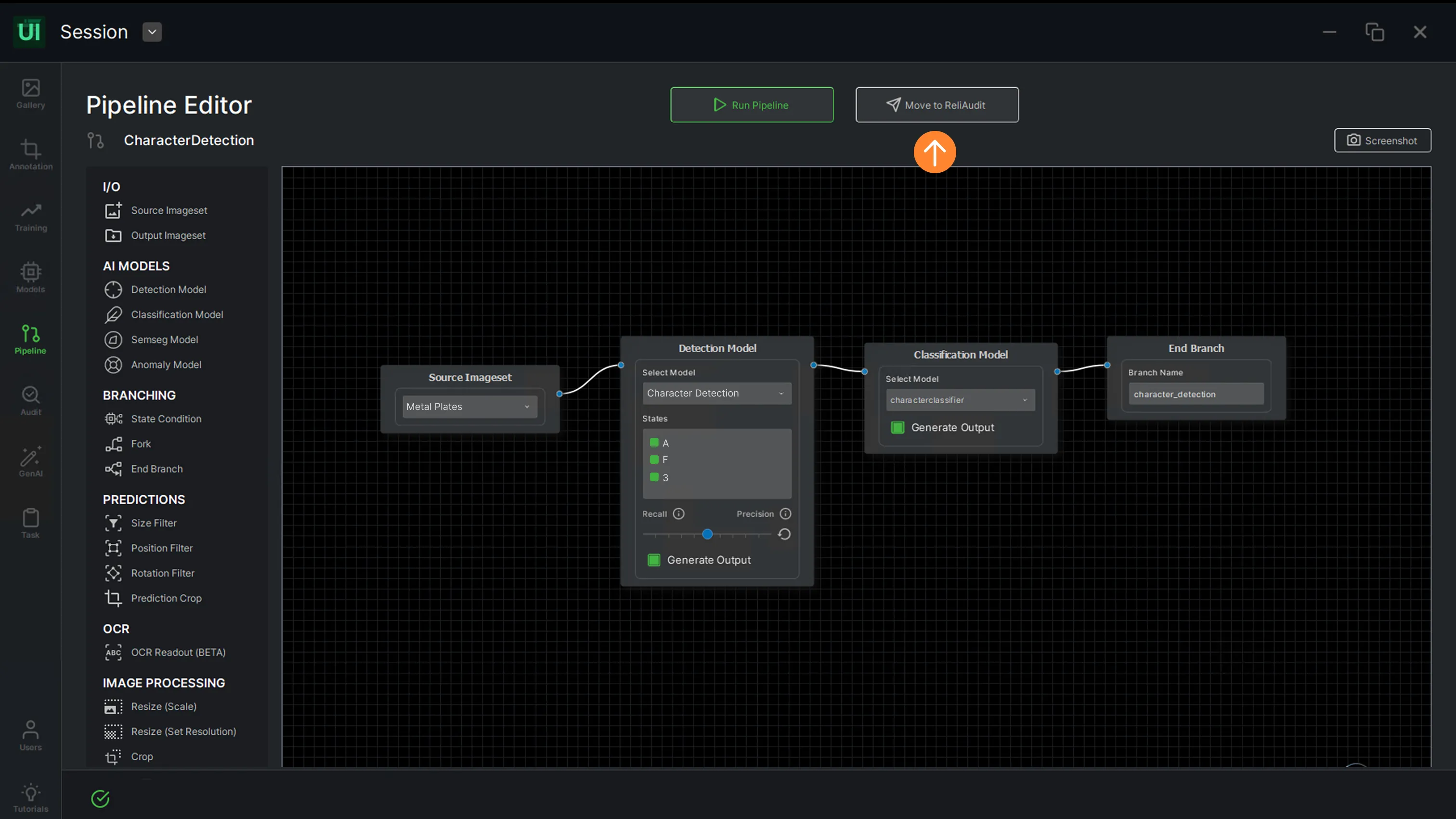
17. If the user prefers to continue with the audit process, go back to the pipeline and add the “End Branch” node.

    

18. Give a name to the end branch, then simply click on the “Move to ReliAudit” button.

    

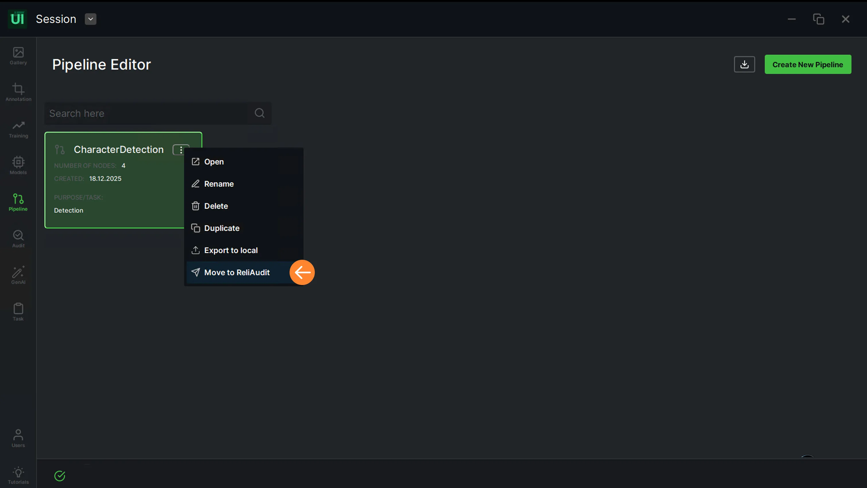
19. Similarly, the user has the option to send the pipeline to the audit by clicking on “Move to ReliAudit” from the “More” menu.

    

Pipeline editor

NLP prompted custom node

ReliVision provides a sophisticated environment for NLP-driven code generation that extends beyond simple automation. This comprehensive workspace ensures that all produced code is immediately operational, verifiable and manageable for technical teams. Users maintain full control to review, modify and validate script logic before completing the integration of any pipeline node.

1. On the Pipeline Editor page, scroll down in the left menu. Click the “Add Custom Node” button to create a custom node.

   

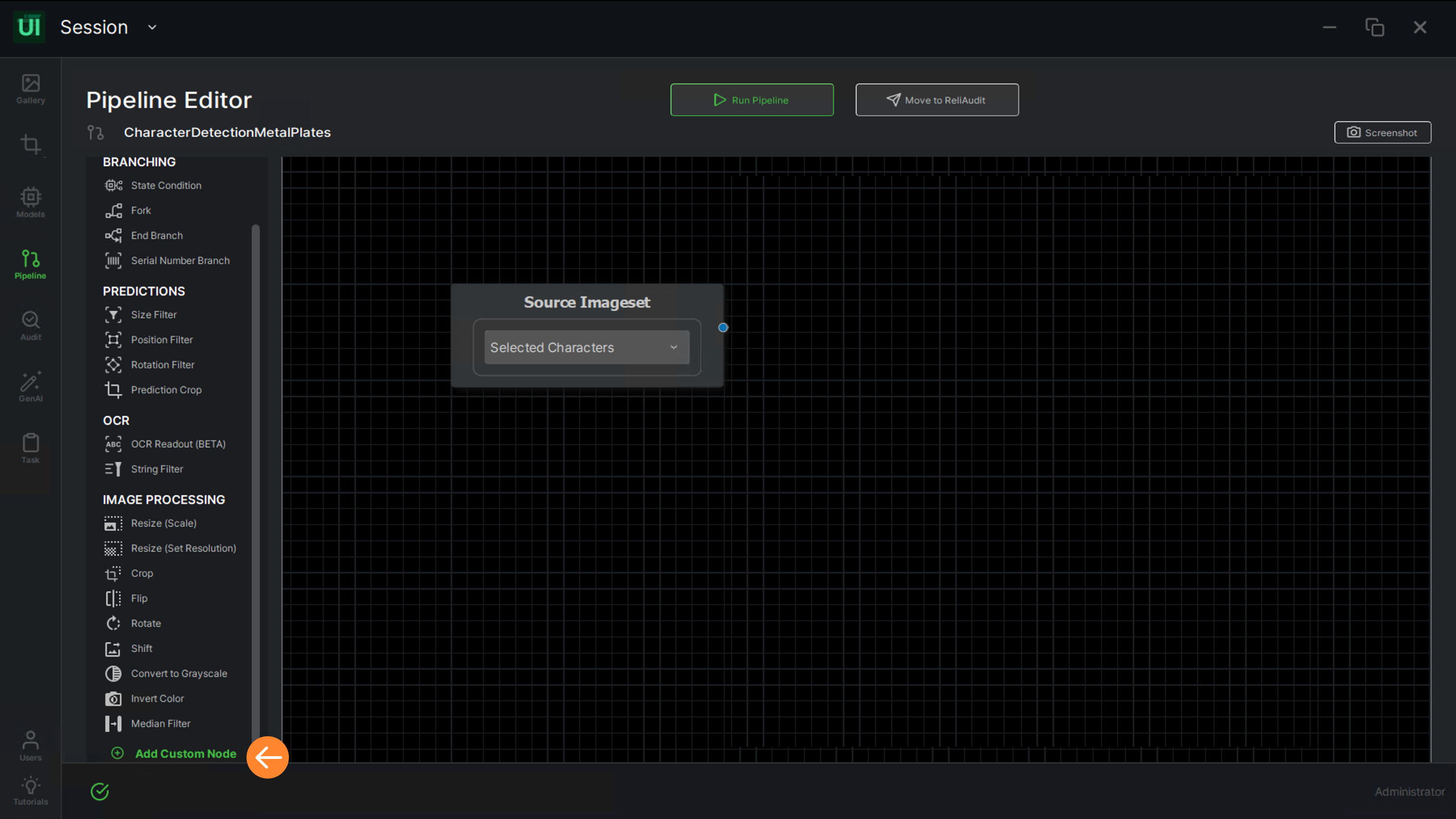
2. Enter a node name and click “Next”.

   

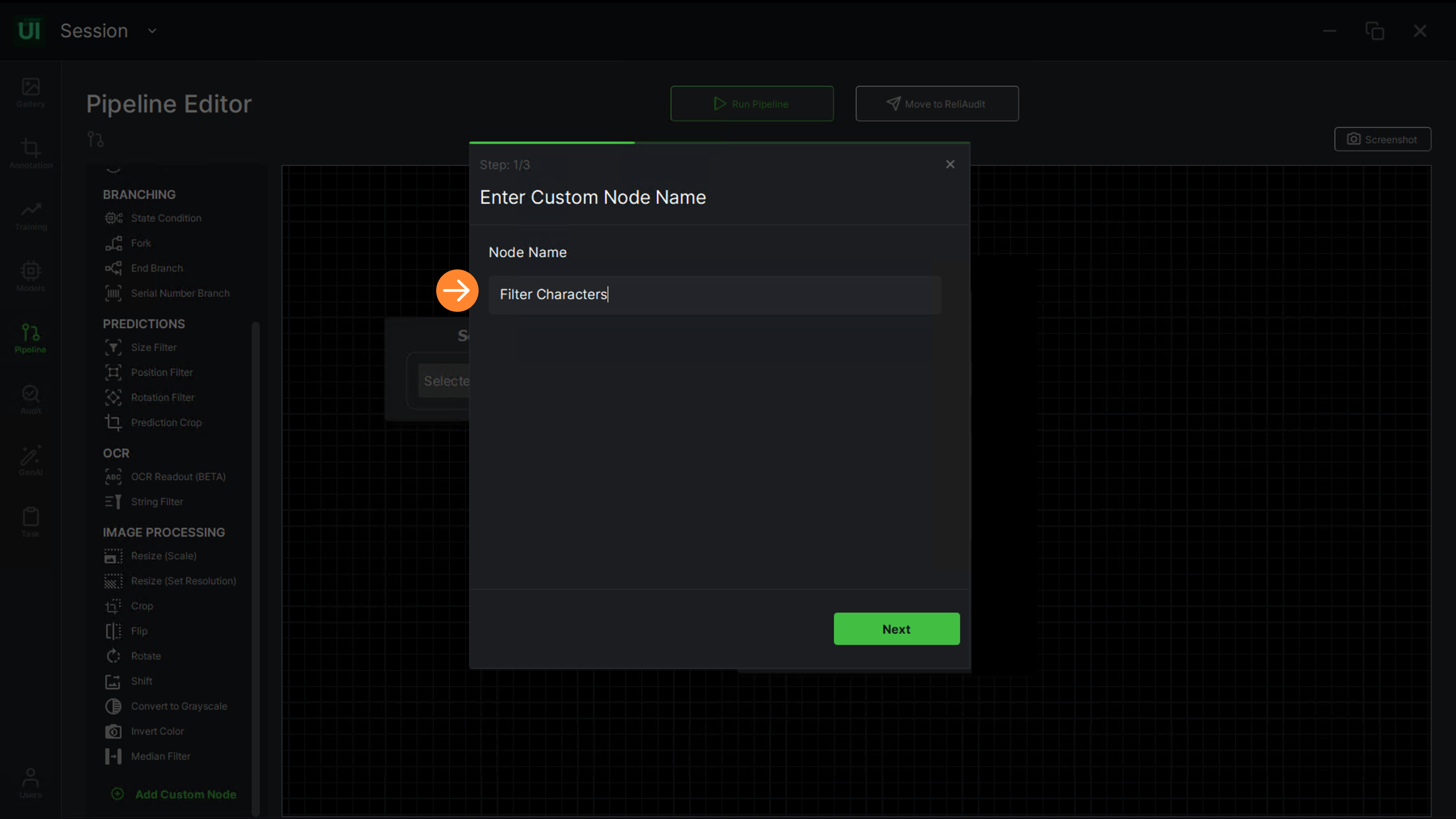
3. Provide a detailed description for automated code generation.

   

4. Optionally, attach a sample image from an available dataset to improve prediction accuracy. Once added, click on “Generate”.

   

5. Once the generation is complete, click on “Next”.

   

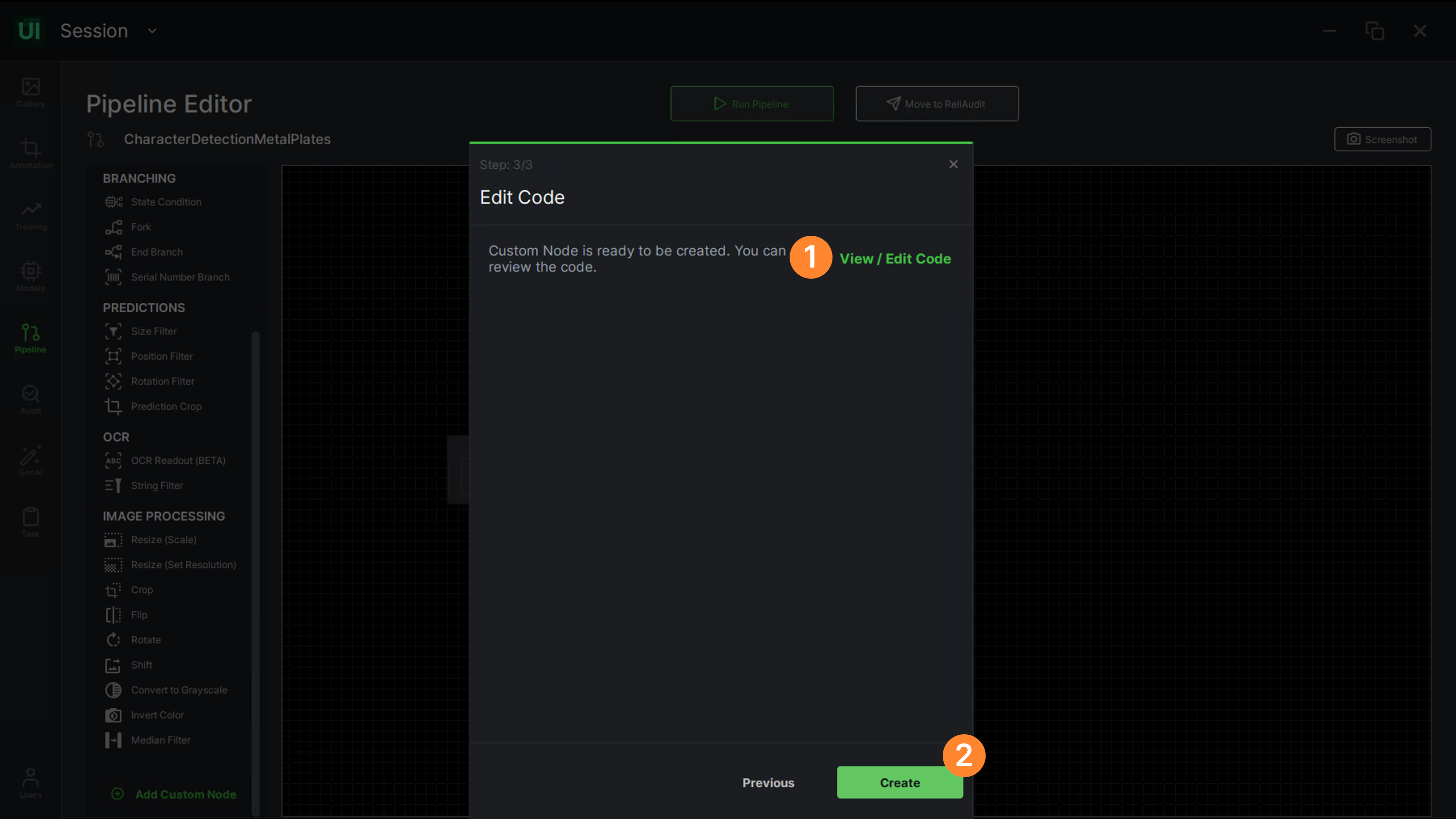
6. Finally, the user can review and edit the generated code by clicking “View/Edit Code” (1) or create the node directly by clicking the “Create” button (2).

   

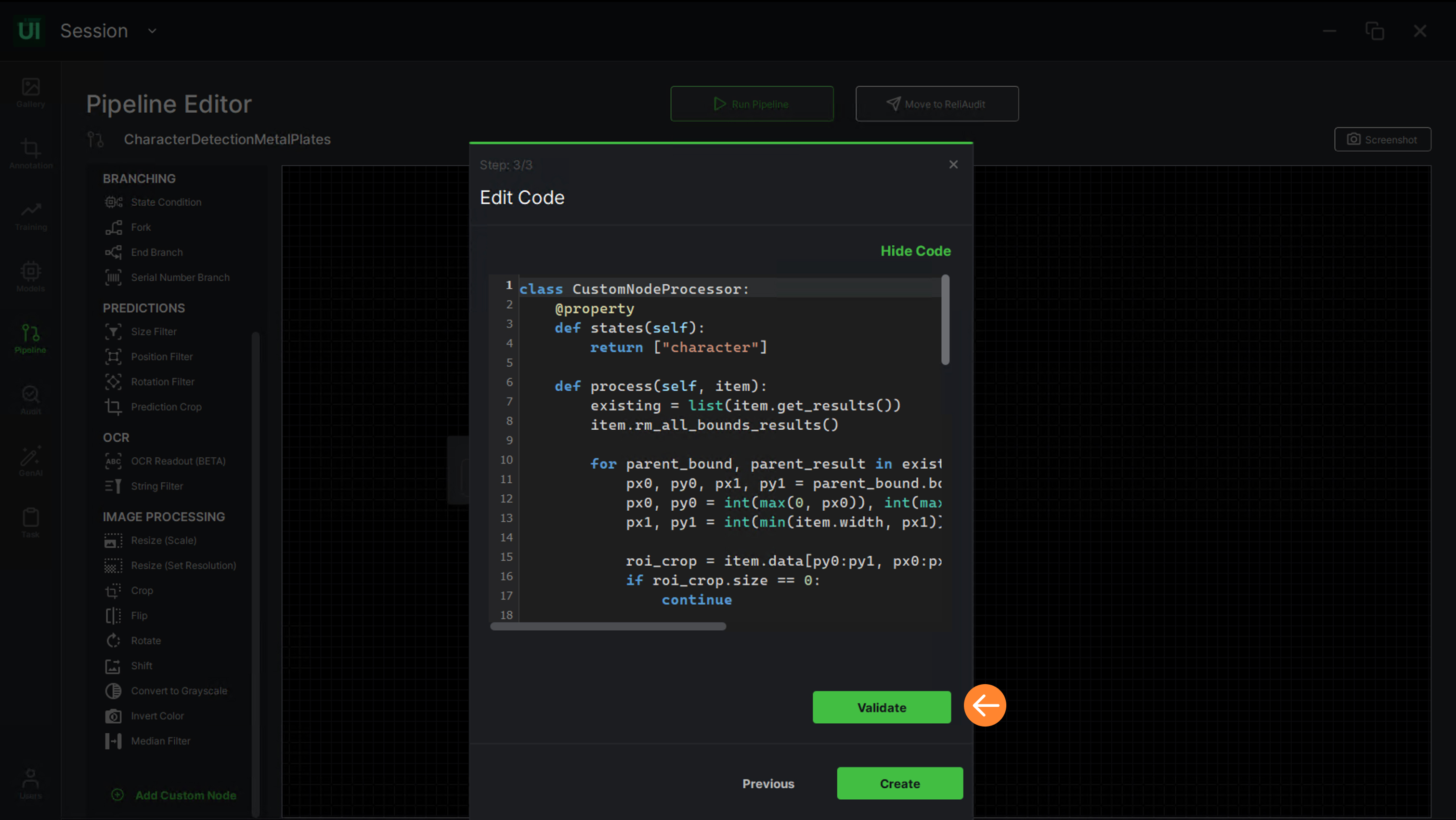
7. The user maintains full control to modify the logic of the script. Should any adjustments be performed, simply select the “Validate” button to confirm the updated code.

   

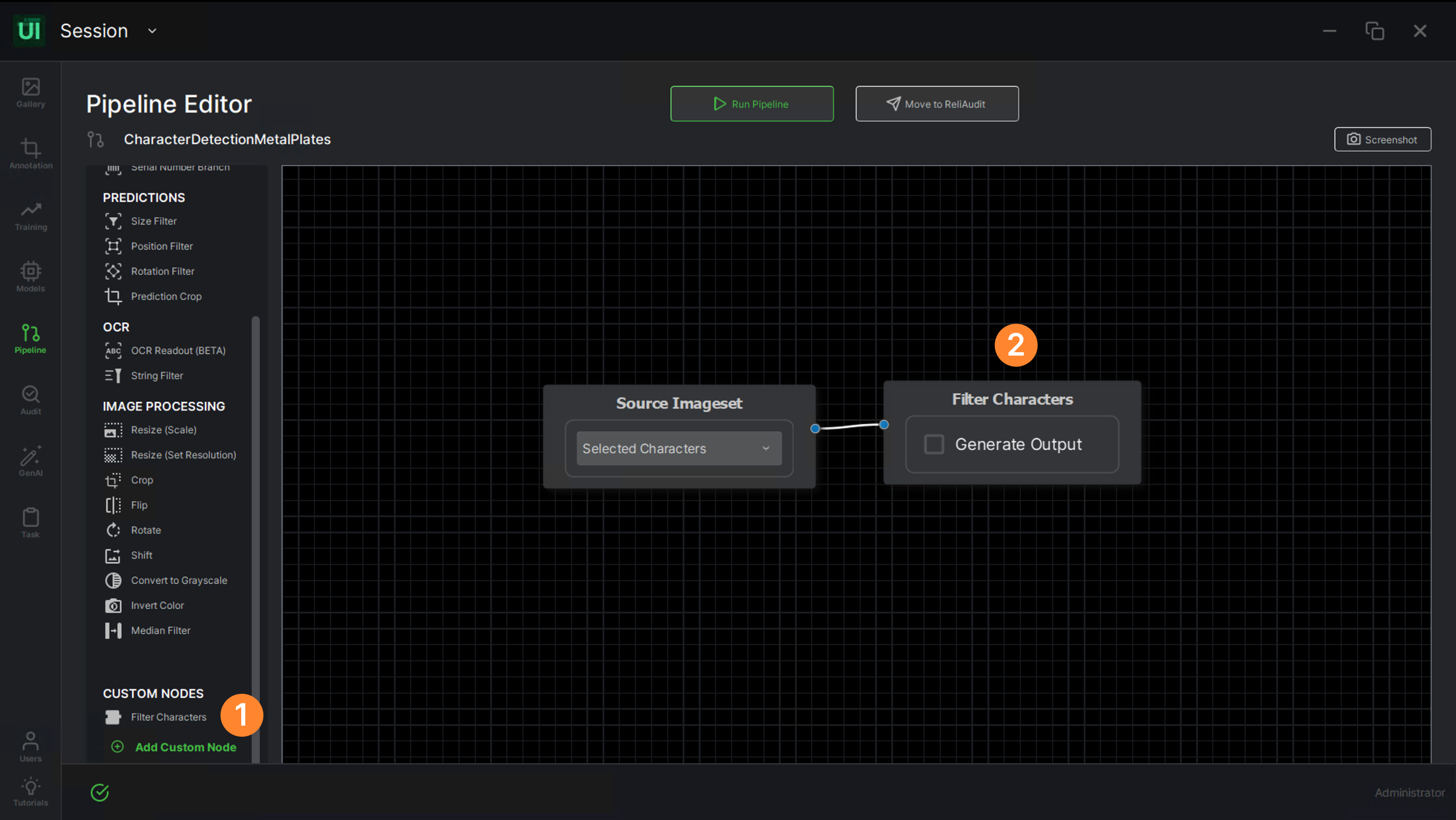
8. Newly created nodes appear in the left menu (1), allowing the user to drag and drop them directly onto the workflow area (2). Once placed, link the node to other relevant blocks (e.g. Source Imageset).

   

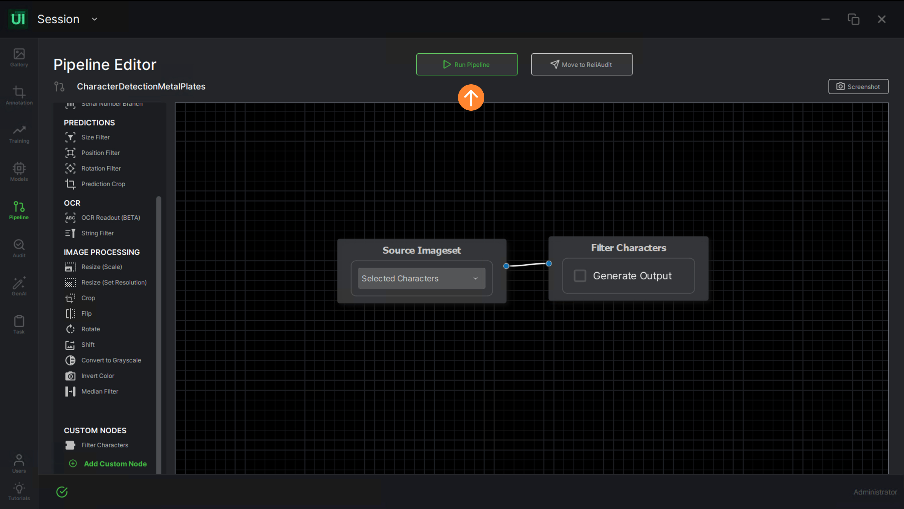
9. Once everything is ready, click on the “Run Pipeline” button on the top.

   

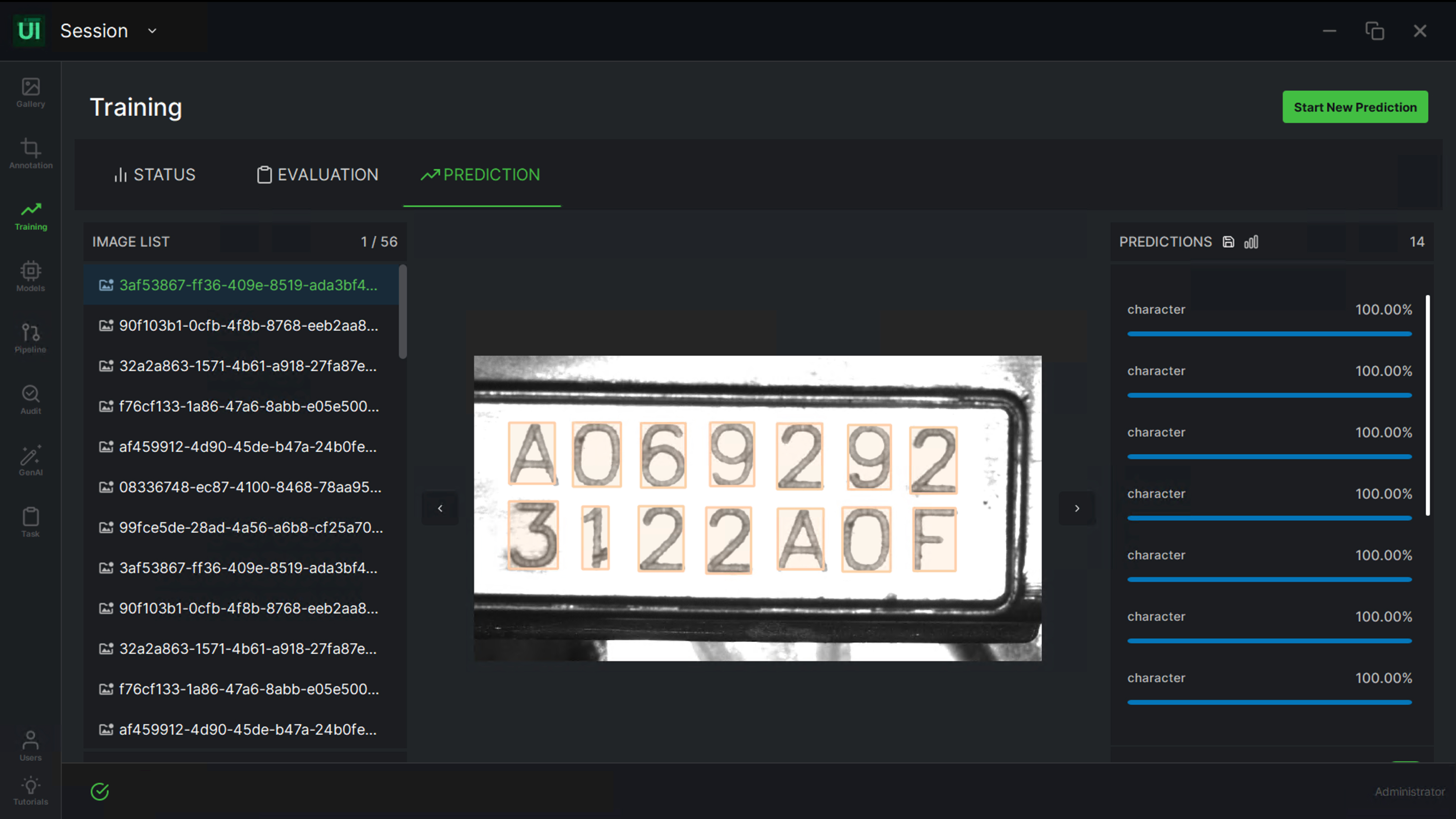
10. The outcomes from the pipeline demonstrate that these custom nodes accurately identify characters according to the specific logic defined within the user's prompt.

    

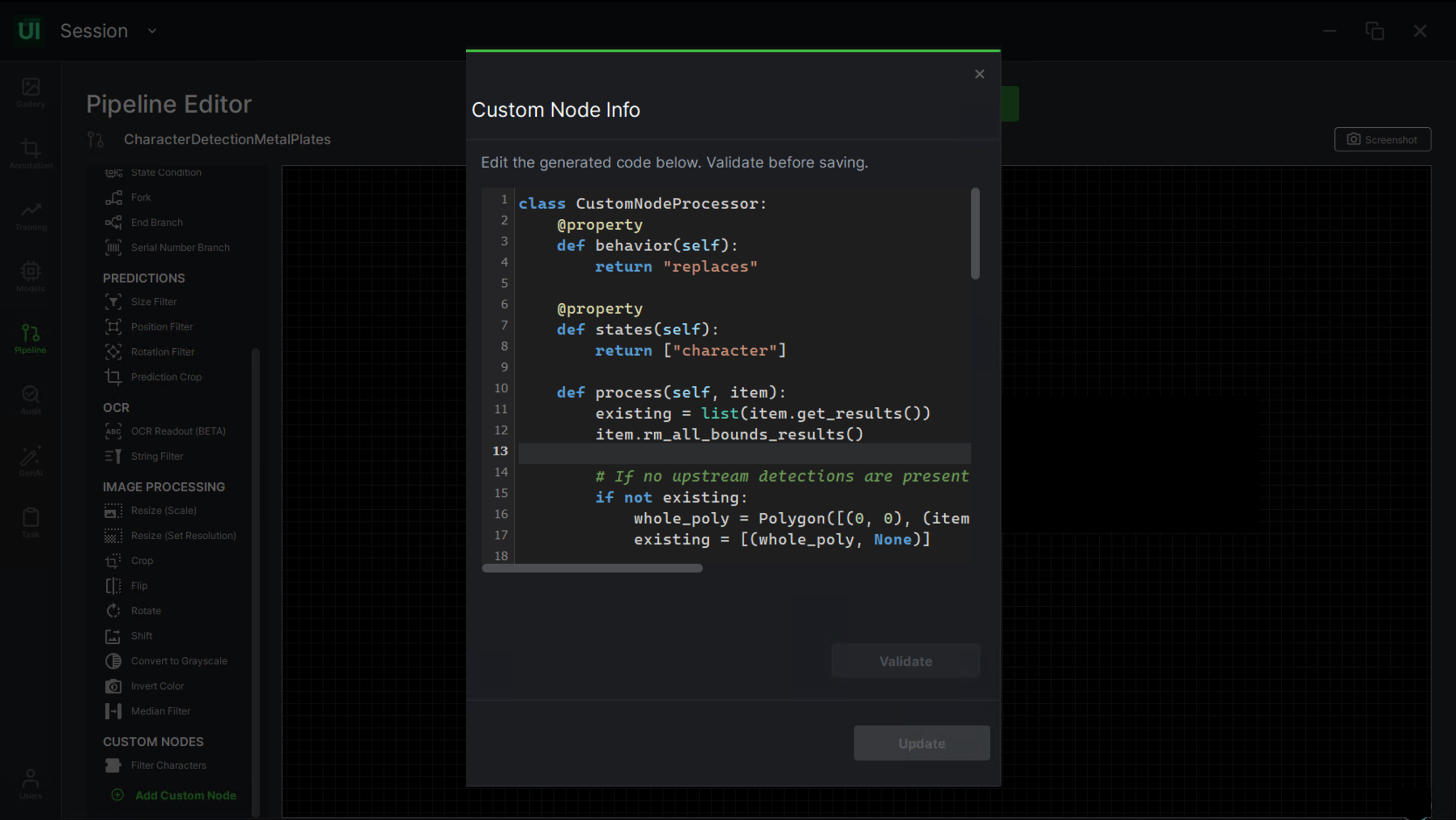
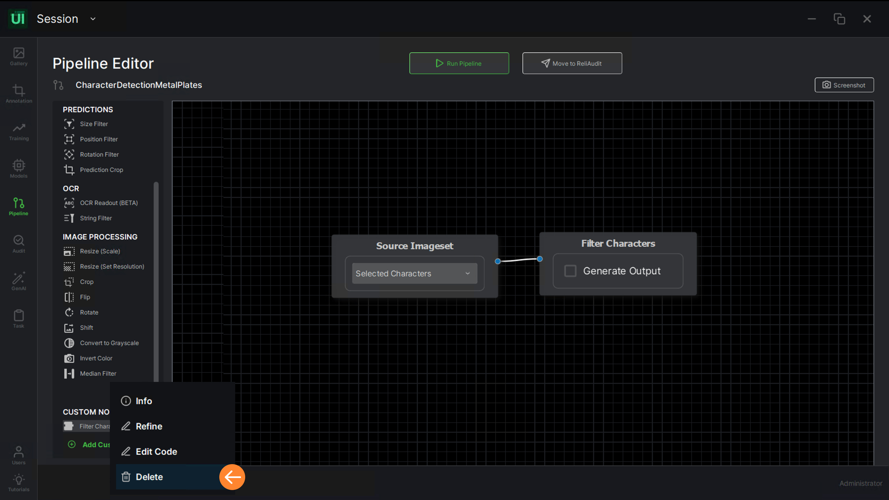
11. To make further modifications, return to the pipeline editor. Right-clicking a custom node will reveal additional options — for example, selecting the “Info” option allows users to preview the custom node prompt.

    

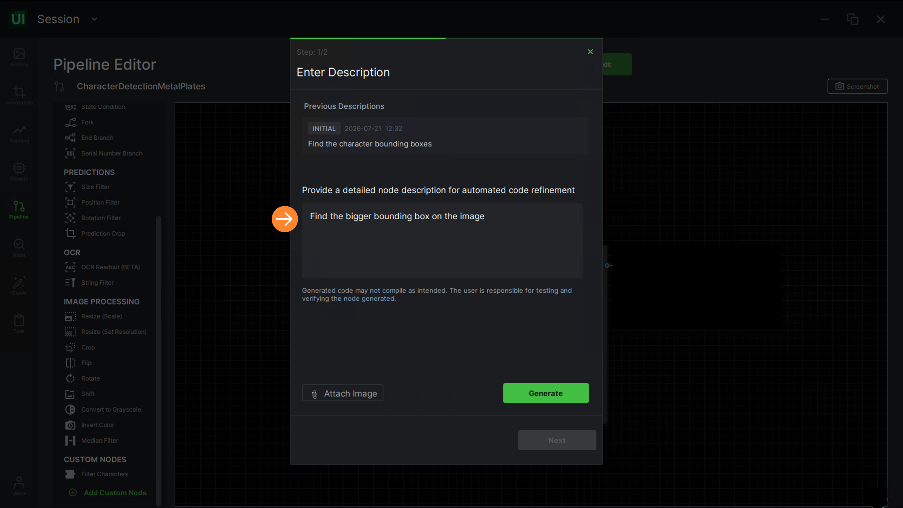
12. Select “Refinement” to incorporate further specifics or clarify requirements.

    

13. Choose the “Edit Code” option to manually modify the code.

    

14. To remove a custom node, choose the “Delete” option.

    

Audit configuration

Create and edit an audit

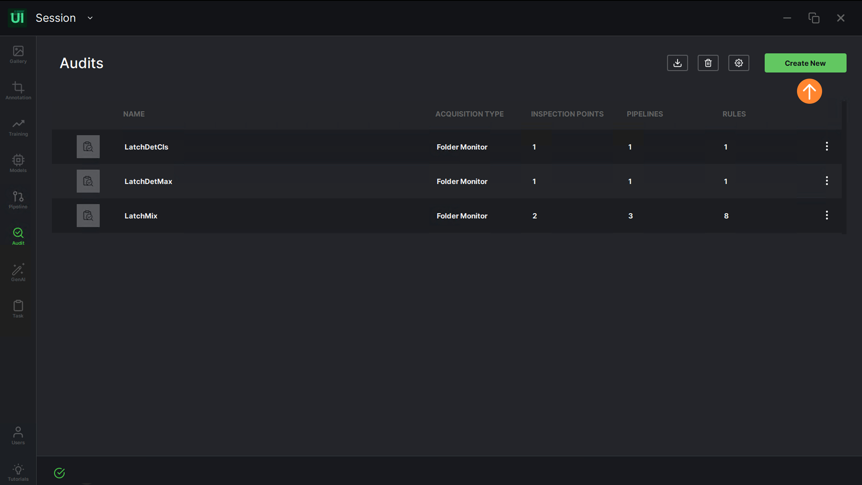
1. Navigate to the “Audit” page and click the “Create” button.

   

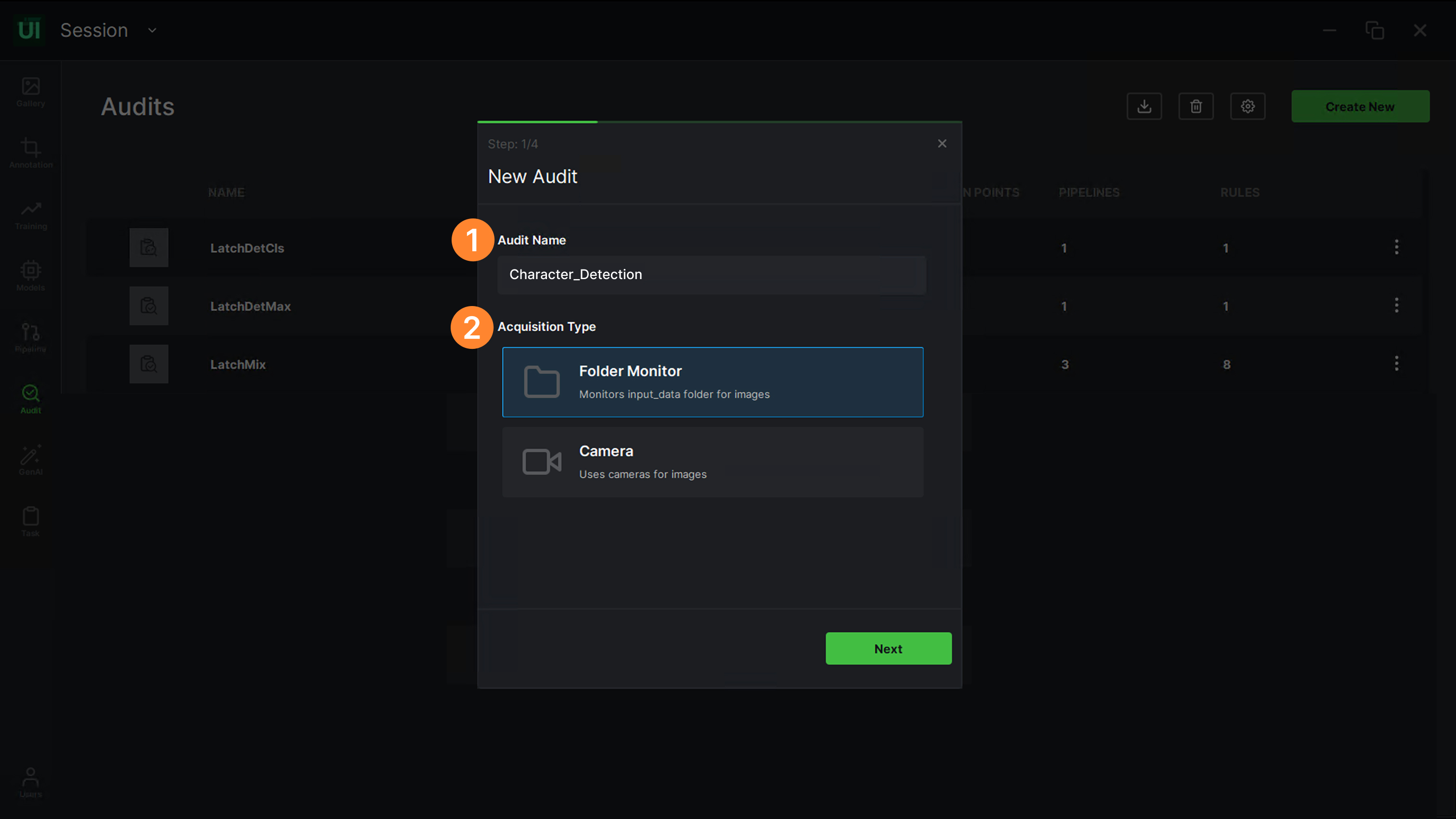
2. Give an audit name (1) and select the acquisition type (2).

   • “Folder Monitor” enables the system to observe the input_data directory for new image files.
   • “Camera” utilizes connected camera hardware to acquire image data.

   

3. Select the pipeline to add to the audit, then click “Next”.

   

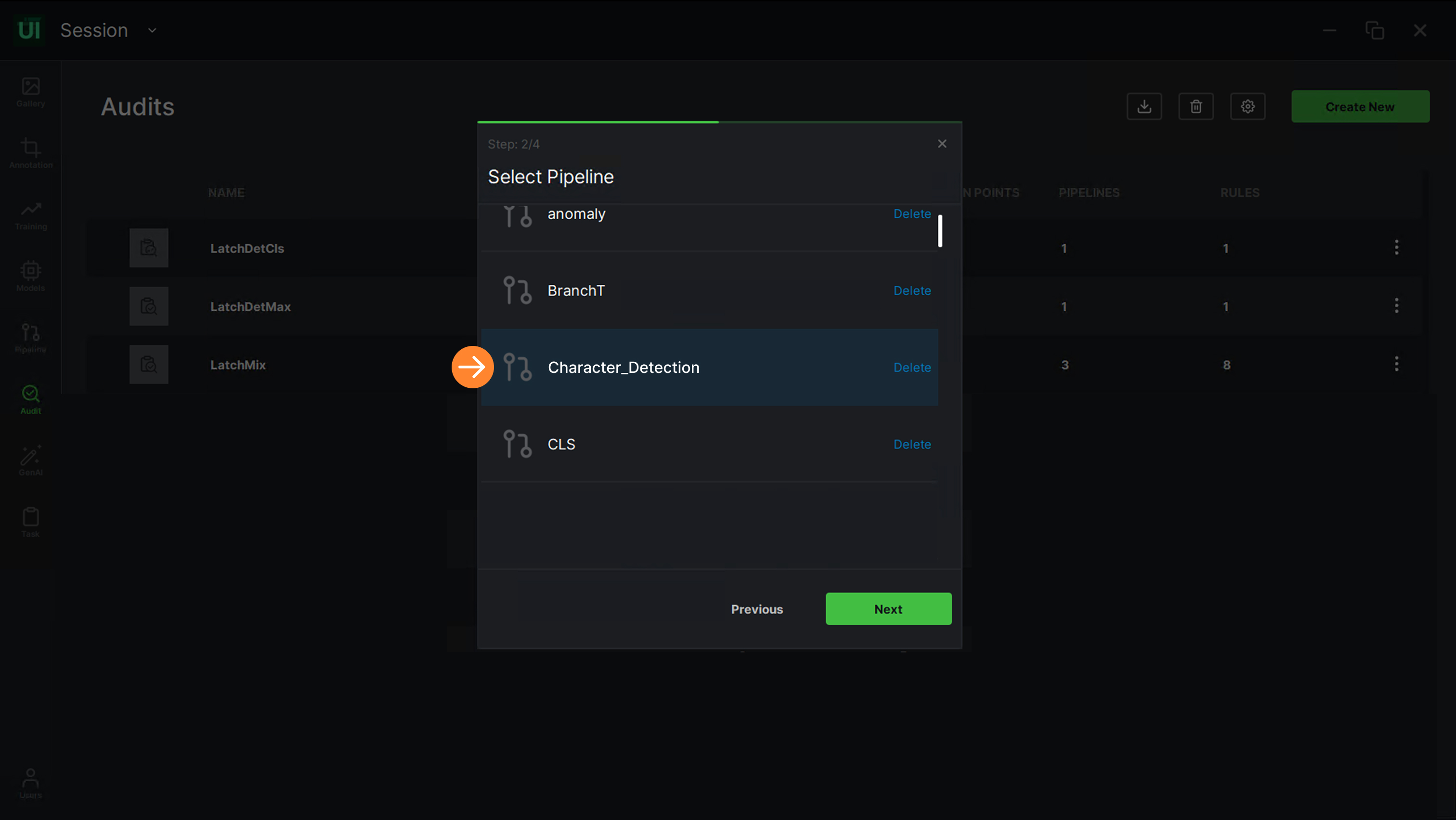
4. Enter a data source name (free text) or select it from the available options to indicate a specific source.

   

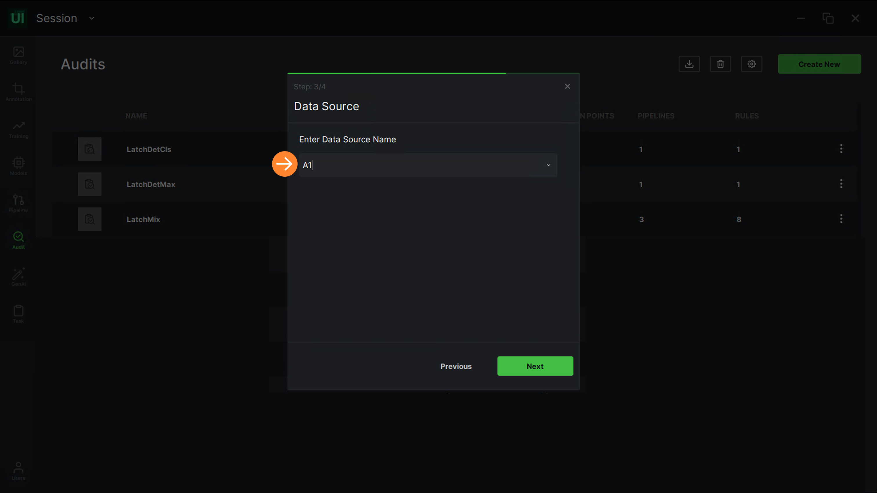
5. Once the new pipeline is added to an audit, you are asked to define the OK rule for that pipeline. The system displays all possible output states and requires you to set the condition per pipeline output state required for the OK decision for that pipeline. The conditions are stated in terms of the number of observations of that state. In the example below, the pipeline has three output states — “3”, “A” and “F”. If the OK decision rule is to have either A, F or 3 detected, the individual output state conditions are set as “A > 0”, “F > 0” and “3 > 0”.

   

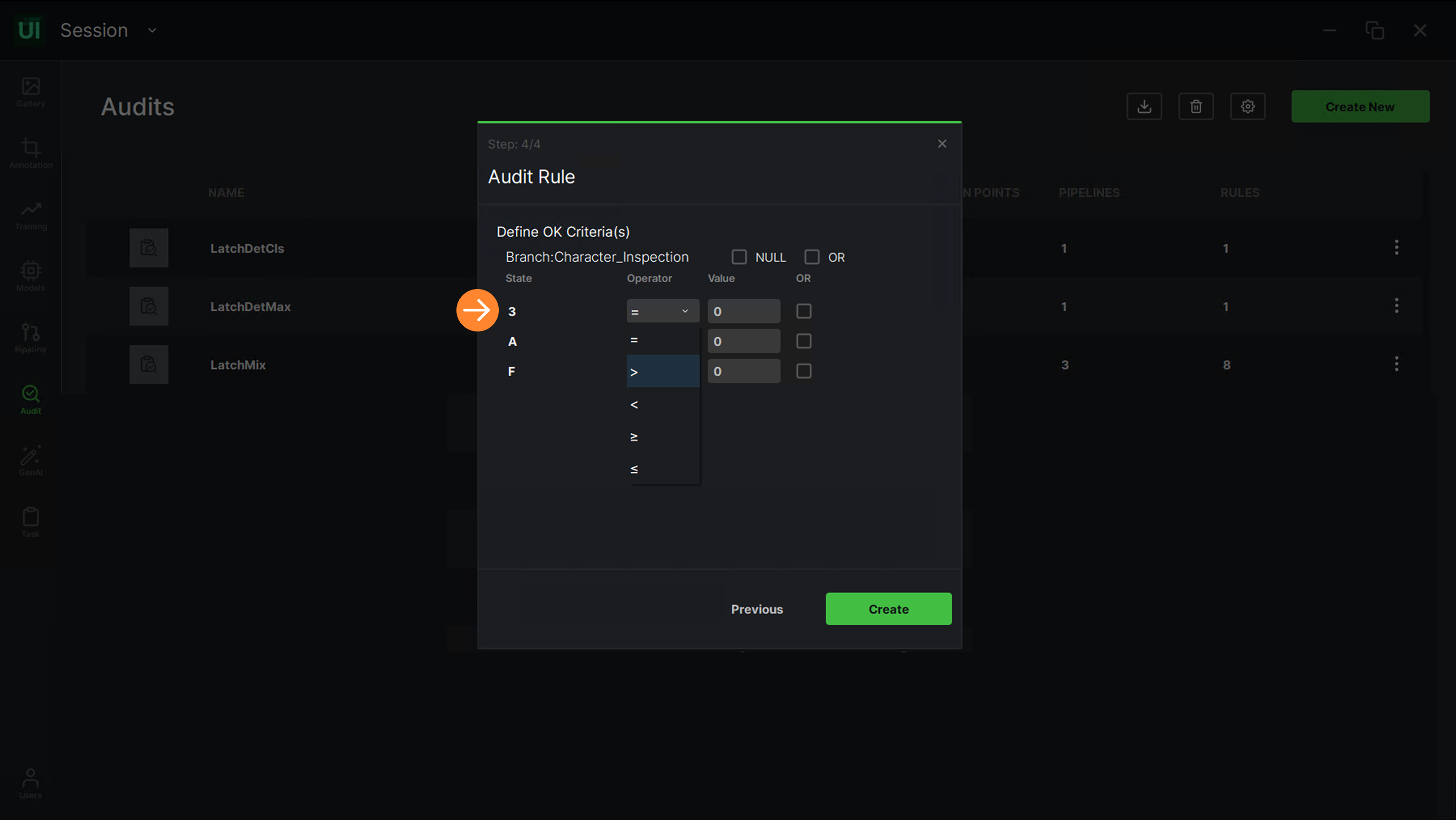
6. When the user chooses the “NULL” checkbox, the corresponding pipeline is designated as null.

   

7. The new audit will be shown in the list together with the existing audits. You can double-click on an audit to open and edit its pipelines' OK decision rules.

   

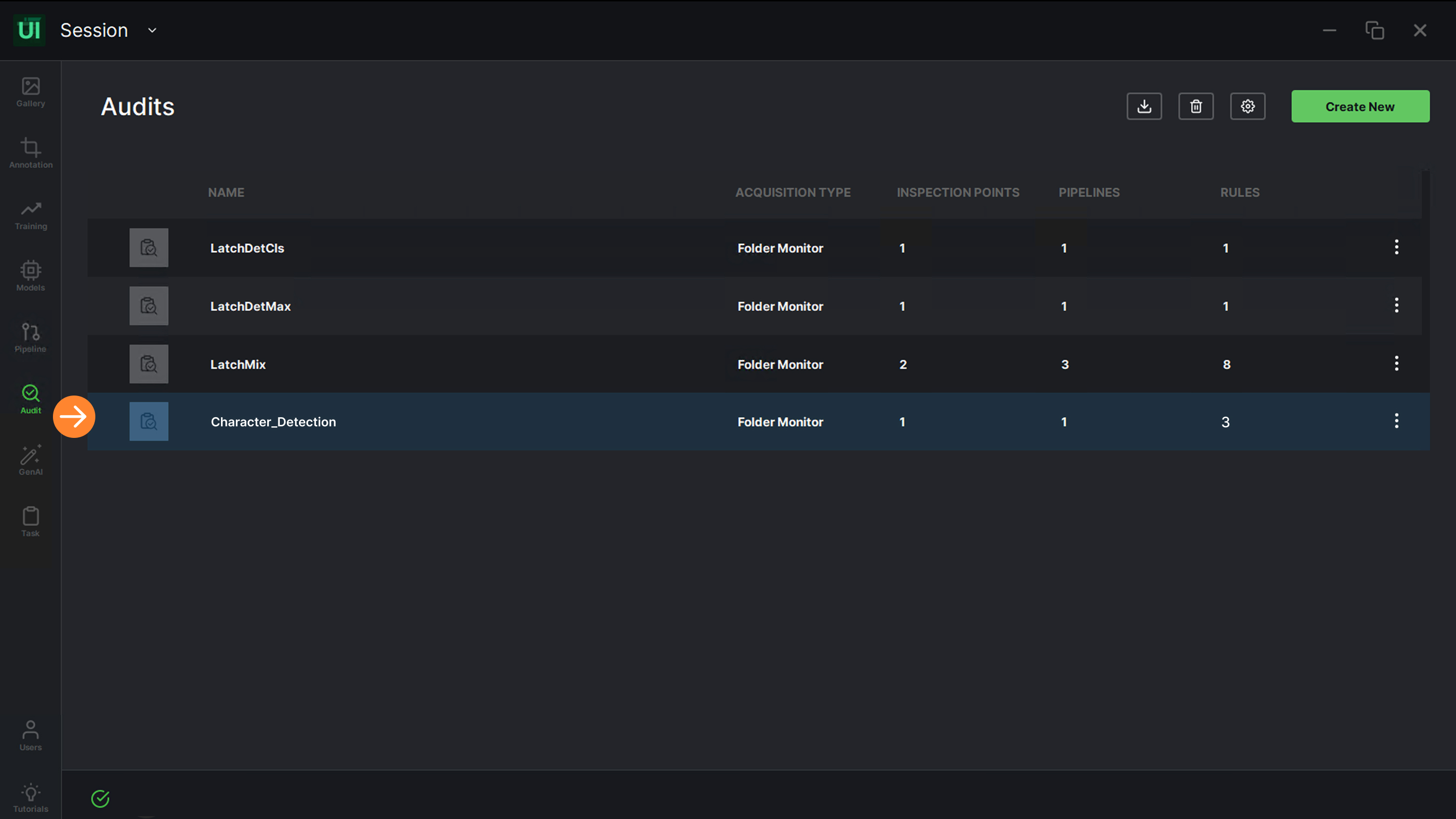
8. The audit details page has two columns: pipelines included in the audit are shown on the left side (1), and the “OK” decision criteria per pipeline are shown on the right side (2). If any criteria is changed, you need to “Save” (3) the change for it to be active.

   

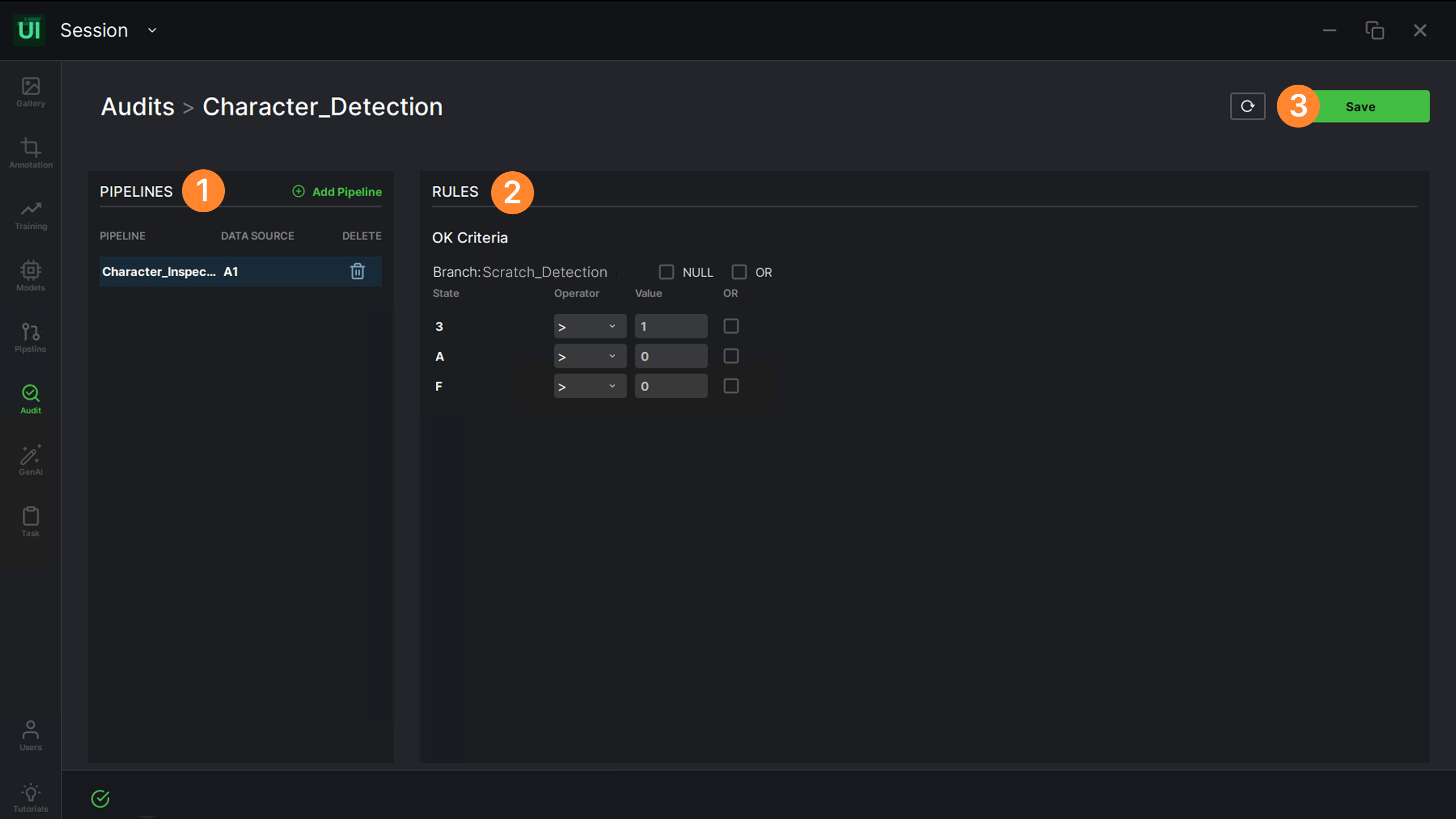
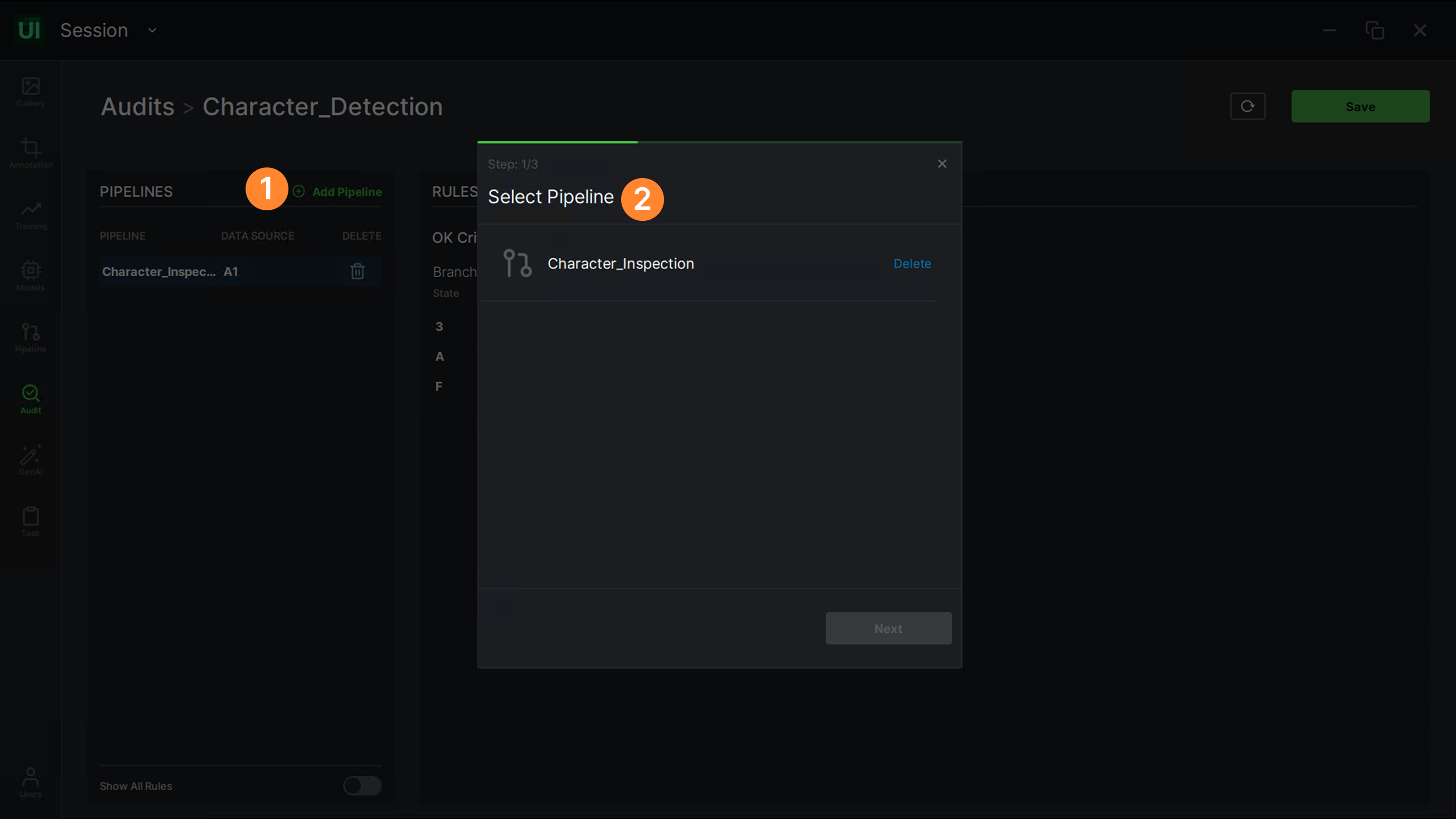
9. If you want to add a new pipeline to an existing audit, click on the “Add Pipeline” button (1), then select a pipeline (2), enter a data source and define the “OK” decision criteria as explained above.

   

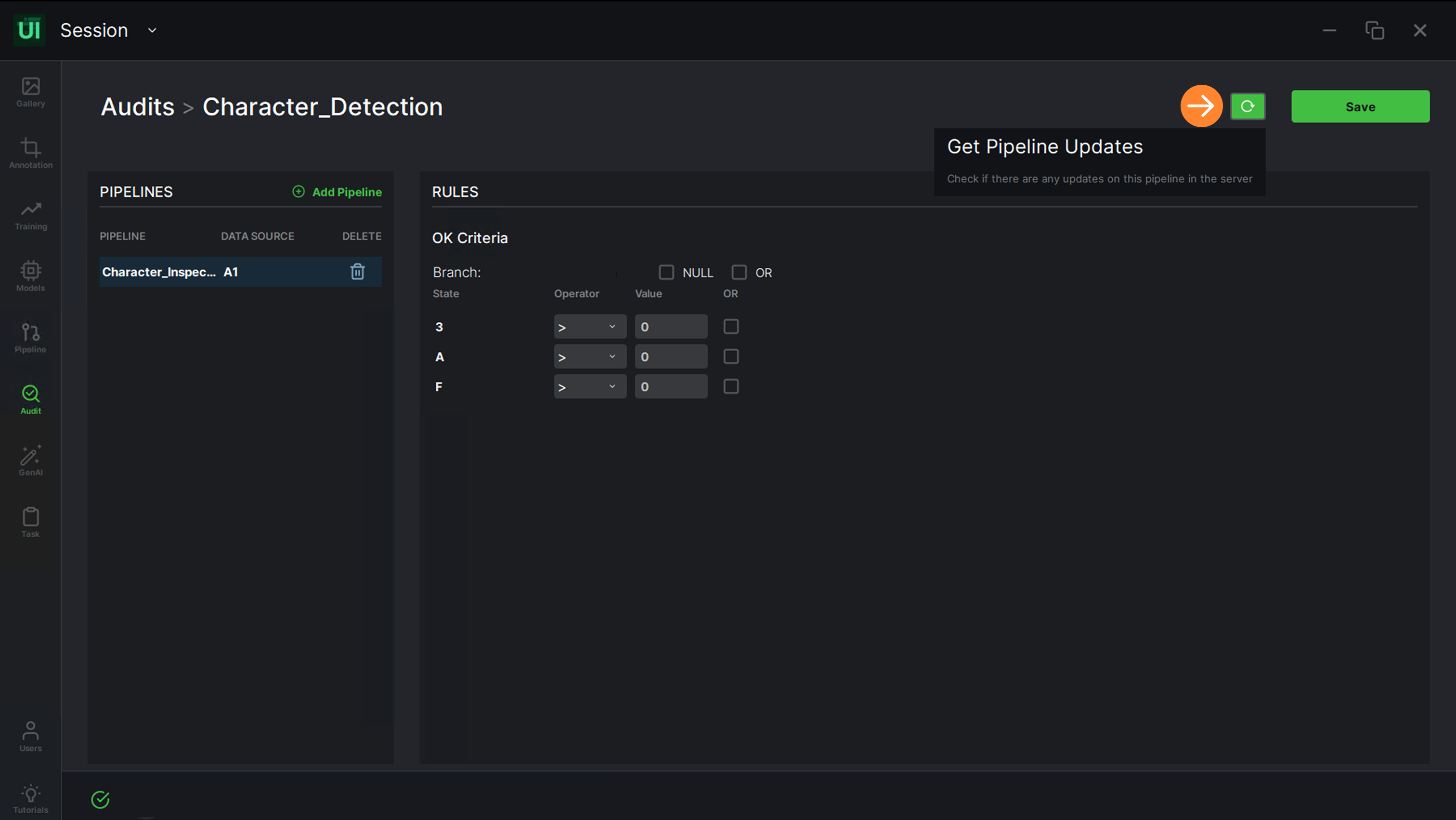
10. To retrieve pipeline updates, click the “Get Pipeline Updates” button.

    

11. To export an audit, click the “More” icon and choose the “Export” option.

    

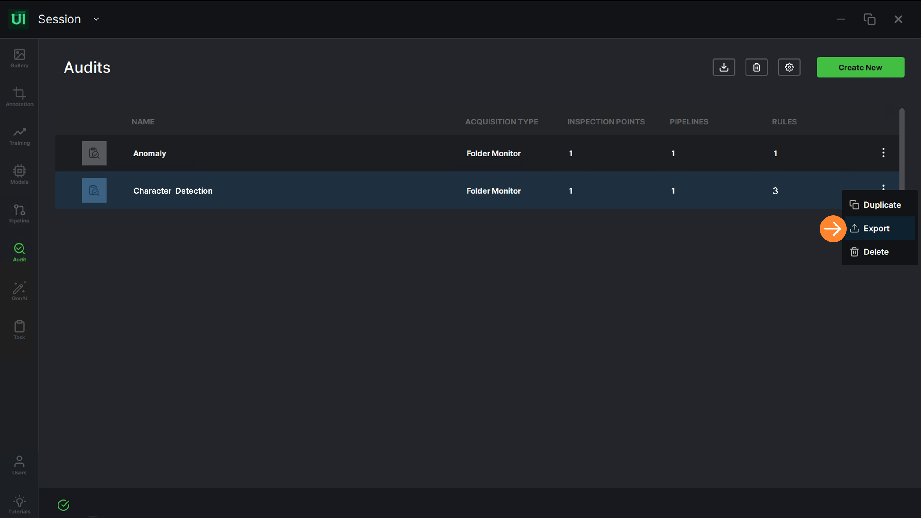
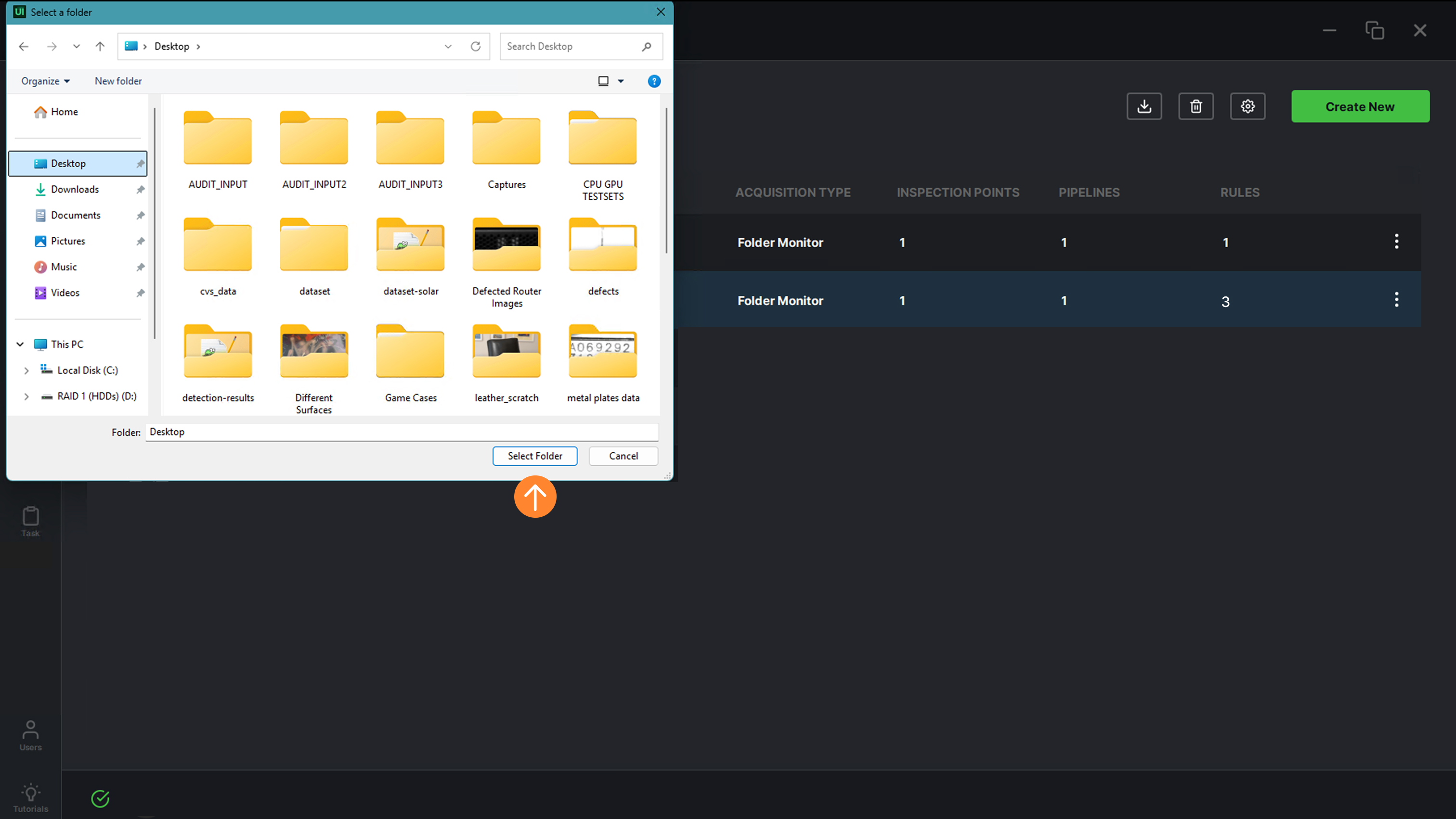
12. Choose a local destination folder where the audit data will be exported and saved.

    

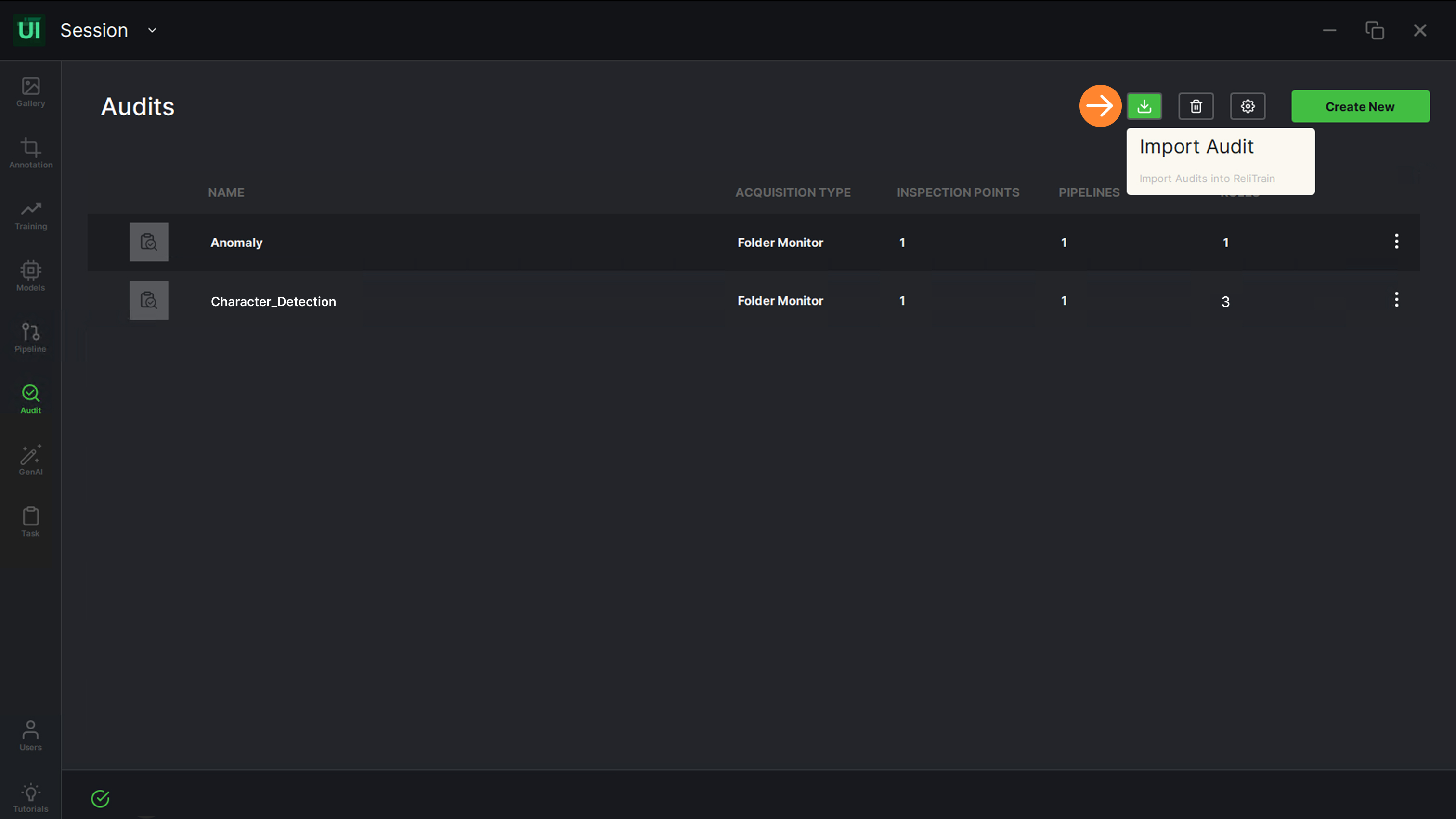
13. To import an audit from your local storage, click on the “Import Audit” button.

    

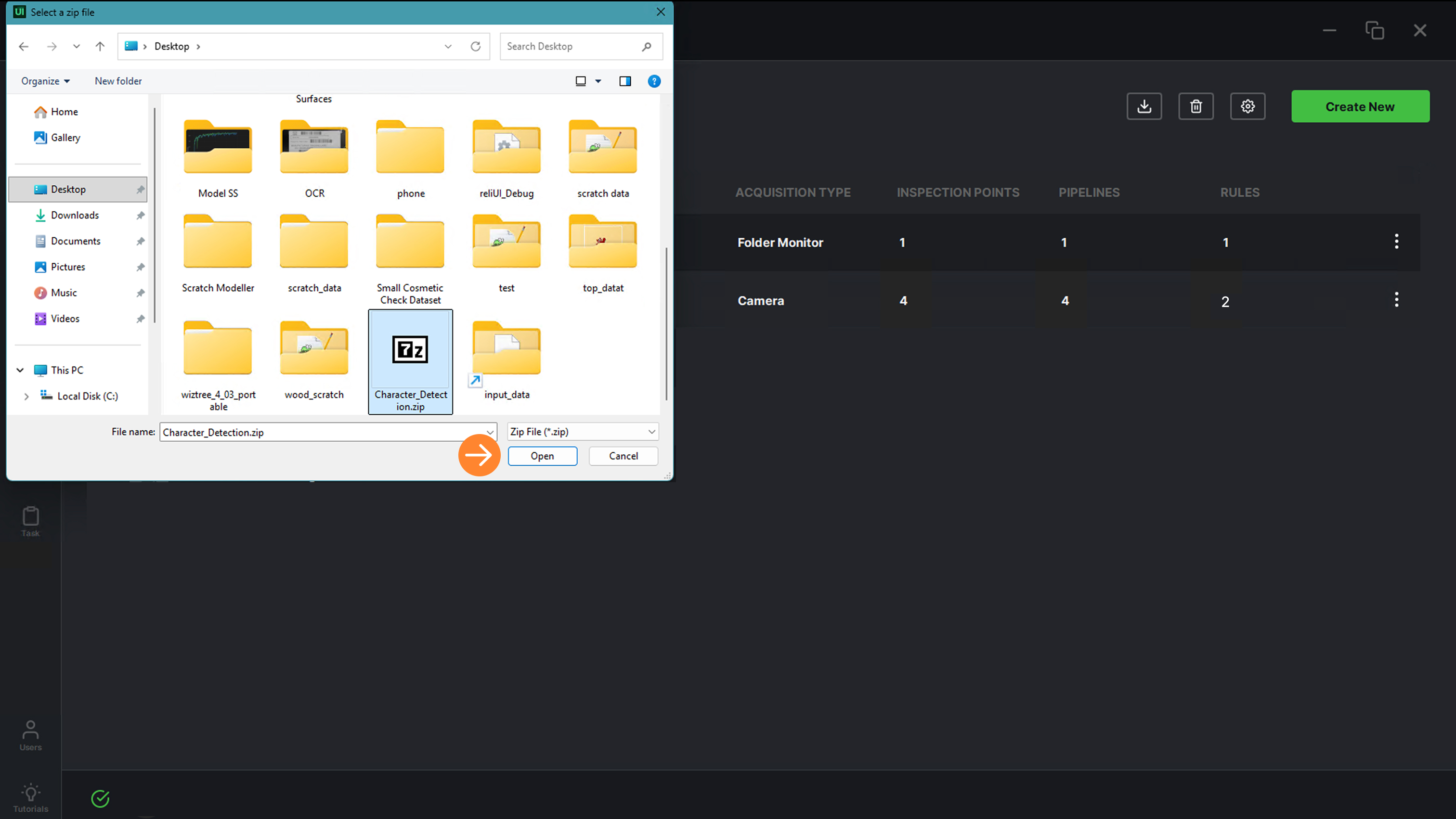
14. Select the audit, then click on “Open”.

    

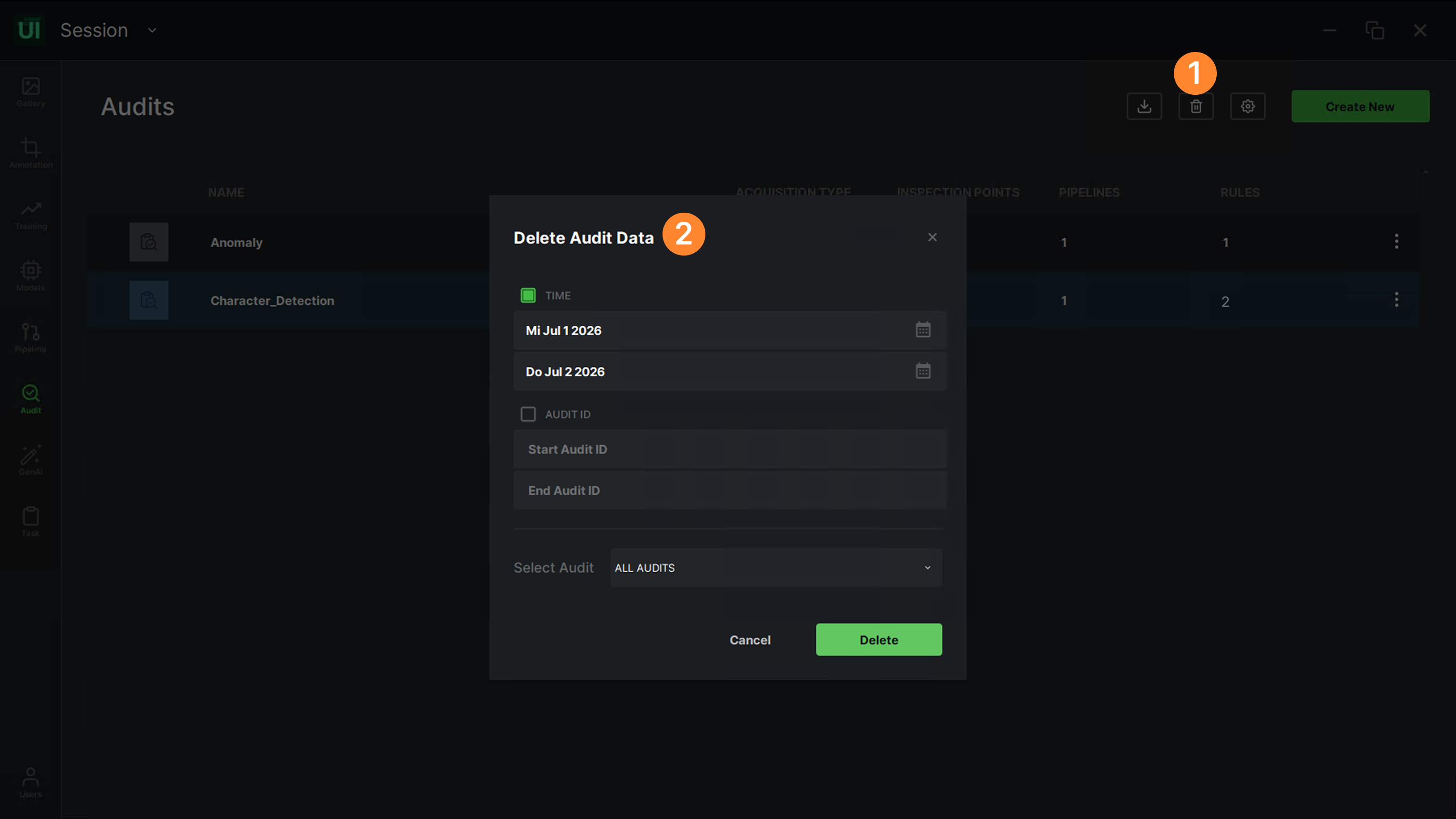
15. To remove previous audit data, click the “Delete Audit History” icon (1). The user may then choose to filter by time, specific audit ID or a particular audit instance (2).

    

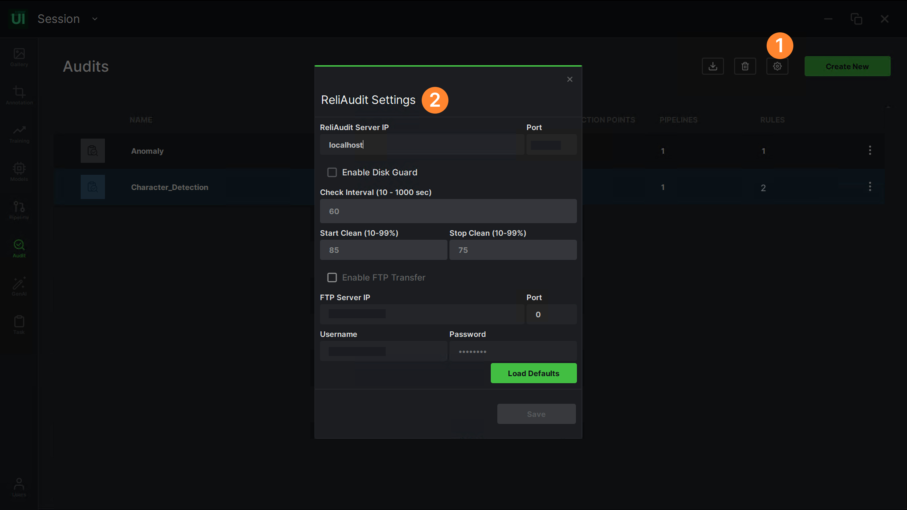
16. To adjust audit configurations, click the “Settings” icon (1). The user can then modify the Server ID, ports and additional parameters (2).

    

Audit configuration

On-prem integration

The edge inference module ReliAudit can be integrated with your external systems — manufacturing, testing, inspection and so on — using five endpoints. Below are the details for using the ReliAudit endpoints for integration with external systems, including data acquisition systems.

• init_audit — Initializes the audit specified by the audit name. Initialization includes loading all required pipelines with AI models and warming up. This call usually takes a couple of seconds, depending on pipelines and models.
• start_audit — Starts a new audit or inspection instance of the specified audit name for the object of interest — a product, say — identified by an ID. The audit name must be the same as the one passed to the last call of init_audit. The product ID identifies the individual object and is displayed in ReliWeb as the “Serial Number”; in ReliAudit there are no constraints on the ID, which is a string. The endpoint returns a unique audit ID.
• add_image — Adds the image specified by file path to the audit specified by an ID. The audit ID must be the one returned by start_audit. Depending on the configuration, each audit can have one or more inspection points and so one or more images; the name of the inspection point is passed to add_image along with the other parameters. ReliAudit processes each image immediately after it is added. After calling start_audit, external data acquisition must call add_image for every inspection point in order to finalize the audit. The final audit result (OK/NOK) is displayed in ReliWeb.
• get_results — Returns the audit results specified by the audit ID, the time interval, the product ID (serial number) or the number of last audits.
• get_status — Returns the list of available audits and the currently initialized audit.